Transforming Quality and Production Conditions into ‘Computable Decision-Making’: 10 Exercise-Keys to Manufacturing Optimization and Machine Learning (No.091–No.100)

This article focuses on Determining process conditions to improve productivity while suppressing defect rates using a fictional resin molding factory as its subject. From gradient descent methods to GPU numerical calculations, we check not just memorizing algorithms, but as a series of decision-making processes involving objective functions, constraints, verification, and operation.

The values handled are fictitious data for explanation purposes. Optimization results should be verified step-by-step within the scope of equipment limits, safety conditions, and quality assurance procedures that are not directly applied to the actual equipment.

[!NOTE] This material is a notebook previously used by Surikoubo (or personally by the representative, Kazuyama), and has been reconstructed, edited, and published with the company’s permission. All data listed is fictional and has no relation whatsoever to real companies, factories, or figures.

Introduction: Practical Challenges in Manufacturing Covered in This Article

When reviewing molding conditions, while raising the temperature stabilizes filling, multiple KPIs compete, such as material degradation and increased power consumption. Furthermore, the minimum predictive model value obtained from historical data does not necessarily guarantee safe driving conditions. In this article, we place objective functions that convert quality loss, cycle time, and energy into monetary terms, and explore candidate conditions within constraints.

Common situations on site

• Experts adjust temperature and pressure little by little, but the basis for judgment is closed to the individual
• Although a quality model was created, the methods for calculating recommended conditions and the approval procedures were not yet well established
• As training data increases, retraining time and selection of computing platforms have become challenges
• Reducing the defect rate alone leads to deterioration in capacity, power, and equipment load

Why is this issue so difficult to judge?

Optimization is not just about calculating the minimum value. The answer varies depending on the unit of the objective function, the scale of the variable, local solution, learning rate, constraints, and model error. What’s important on the ground is not only the recommended value itself but also being able to explain the Under which assumptions and within which constraints, how much improvement is achieved over current conditions?.

Overview of Exercise covered this time

Representative optimization algorithms are compared from No.091 to No.096, and safety and capability constraints are added in No.097. No.098 integrates automatic differentiation, No.099 on GPU usage, and No.100 on numerical calculations into checklists for business implementation.

Preparing the Python environment

Optimize with NumPy and SciPy, visualize with pandas tables, and visualize with matplotlib. In No.098 to No.099, PyTorch automatic differentiation and device determination are used. Fix random number seeds so that results can be reproduced in the same environment.

%matplotlib inline
import platform
import time
import numpy as np
import pandas as pd
import matplotlib
import matplotlib.pyplot as plt
from scipy import optimize
import torch

SEED = 42
rng = np.random.default_rng(SEED)
torch.manual_seed(SEED)
plt.rcParams["figure.figsize"] = (7, 4)
plt.rcParams["axes.unicode_minus"] = False

print(f"Python: {platform.python_version()}")
print(f"NumPy: {np.__version__}, pandas: {pd.__version__}")
print(f"Matplotlib: {matplotlib.__version__}, PyTorch: {torch.__version__}")

Python: 3.13.1
NumPy: 2.5.1, pandas: 3.0.3
Matplotlib: 3.11.0, PyTorch: 2.13.0

Creation of Fictional Data

Assume $x_1=(T-210)/10$, $x_2=(P-80)/10$, which standardizes temperature $T$ (°C) and holding pressure $P$ (MPa), as explanatory variables. The observed quality loss score should include deviations from the optimal range, interaction between temperature and pressure, lot differences, and measurement noise. It generates 240 lots for learning and another 80 lots for evaluation.

The smooth proxy objective function for optimization is as follows.

$$J(x_1,x_2)=45(x_1-0.8)^2+30(x_2+0.4)^2+12(x_1-0.8)(x_2+0.4)+18.$$

This is considered a simplified model of total loss calculated by converting quality, time, and energy into monetary terms.

def objective(x):
    u, v = x[0] - 0.8, x[1] + 0.4
    return 45*u**2 + 30*v**2 + 12*u*v + 18

def gradient(x):
    u, v = x[0] - 0.8, x[1] + 0.4
    return np.array([90*u + 12*v, 60*v + 12*u])

def hessian(_x):
    return np.array([[90.0, 12.0], [12.0, 60.0]])

n_train, n_test = 240, 80
X_all = rng.uniform([-2.0, -2.0], [2.0, 2.0], size=(n_train+n_test, 2))
lot_effect = rng.normal(0, 1.5, n_train+n_test)
y_all = np.array([objective(x) for x in X_all]) + lot_effect + rng.normal(0, 2.0, n_train+n_test)
X_train, X_test = X_all[:n_train], X_all[n_train:]
y_train, y_test = y_all[:n_train], y_all[n_train:]
process_df = pd.DataFrame({
    "temperature_C": 210 + 10*X_train[:, 0],
    "holding_pressure_MPa": 80 + 10*X_train[:, 1],
    "loss_score": y_train,
})
display(process_df.head().round(2))
print(f"Learning: {len(X_train)}lot / Reception: {len(X_test)}lot")

	temperature_C	holding_pressure_MPa	loss_score
0	220.96	77.56	22.47
1	224.34	87.89	86.38
2	193.77	99.02	374.53
3	220.45	91.44	97.72
4	195.12	78.02	253.07

Learning: 240 lots / Evaluation: 80 lots

No.091: Slope Descent Method

Meaning in Practice

The gradient descent method is a fundamental technique that iteratively updates process conditions in the direction where losses are minimized. Since the number of trials, the range of changes per change, and stopping conditions can be clearly specified, it forms a foundation for sharing the approach to process condition exploration.

Approach to Analysis and Modeling

The update formula is $x_{k+1}=x_k-\eta\nabla J(x_k)$. If the learning rate $\eta$ is too low, it is slow; if too high, it diverges. If the units of variables differ, if not standardized, only one variable will be overrenewed.

Check with Python

def gradient_descent(x0, lr=0.015, n_iter=40):
    x = np.array(x0, dtype=float)
    hist = []
    for k in range(n_iter):
        hist.append((k, *x, objective(x), np.linalg.norm(gradient(x))))
        x -= lr * gradient(x)
    return pd.DataFrame(hist, columns=["iteration", "x1", "x2", "loss", "grad_norm"])

gd = gradient_descent([-1.5, 1.5])
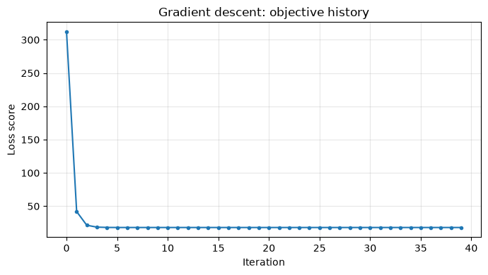
display(gd.iloc[[0, 1, 2, 5, 10, -1]].round(4))
fig, ax = plt.subplots()
ax.plot(gd["iteration"], gd["loss"], marker="o", markersize=3)
ax.set_title("Gradient descent: objective history")
ax.set_xlabel("Iteration"); ax.set_ylabel("Loss score")
ax.grid(True, alpha=0.3); plt.tight_layout(); plt.show()

	iteration	x1	x2	loss	grad_norm
0	0	-1.5000	1.5000	311.9100	203.4566
1	1	1.2630	0.2040	41.9469	64.3419
2	2	0.5292	-0.4229	21.3896	25.0749
5	5	0.8174	-0.3936	18.0162	1.7479
10	10	0.7998	-0.4001	18.0000	0.0210
39	39	0.8000	-0.4000	18.0000	0.0000

Reading the results

At a learning rate of 0.015, total loss decreases with iterations, and the gradient norm decreases. When adopting, not only the final value but also the monotonicity of losses, gradient norms, and iteration limits are recorded in the log. To ensure that proxy functions do not fall outside the range representing the actual process, the search range must also be set.

No.092: Optimization by Newton’s Method

Meaning in Practice

The Newtonian method uses not only gradients but also curvature to efficiently solve problems where the slope of the loss plane varies depending on the direction. It is effective when the number of experiments is expensive and candidates are needed with few iterations.

Approach to Analysis and Modeling

$x_{k+1}=x_k-H(x_k)^{-1}\nabla J(x_k)$ update. $H$ is Hessian. In quadratic functions, theoretically, the minimum point is reached in one pass, but in non-convex problems, the Hessian may not be positively definite, requiring attenuation and confidence regions.

Check with Python

x_newton = np.array([-1.5, 1.5])
newton_rows = []
for k in range(3):
    newton_rows.append([k, *x_newton, objective(x_newton), np.linalg.norm(gradient(x_newton))])
    step = np.linalg.solve(hessian(x_newton), gradient(x_newton))
    x_newton -= step
newton_df = pd.DataFrame(newton_rows, columns=["iteration", "x1", "x2", "loss", "grad_norm"])
display(newton_df.round(6))

	iteration	x1	x2	loss	grad_norm
0	0	-1.5	1.5	311.91	203.456629
1	1	0.8	-0.4	18.00	0.000000
2	2	0.8	-0.4	18.00	0.000000

Reading the results

Since the objective function this time is a quadratic function with a positive constant Hessian, it reaches the theoretical minimum point $(0.8,-0.4)$ in a single update. Real-world quality models are not necessarily quadratic functions. It is necessary to check Hessian eigenvalues, post-step losses, boundary deviations, and design that unconditionally accepts all steps.

No.093: Quasi-Newtonian Method

Meaning in Practice

As the number of variables increases, Hessian’s derivation and calculations become heavier. Quasi-Newtonian methods such as BFGS approximate the inverse Hessian from gradient changes, achieving both practical convergence speed and computational complexity.

Approach to Analysis and Modeling

BFGS learns curvature from update differences $s_k=x_{k+1}-x_k$ and gradient differences $y_k=\nabla J(x_{k+1})-\nabla J(x_k)$. $s_k^Ty_k>0$ is a key condition for stable updates. Here, we use verified scipy.optimize.minimize.

Check with Python

bfgs_trace = []
res_bfgs = optimize.minimize(
    objective, x0=[-1.5, 1.5], jac=gradient, method="BFGS",
    callback=lambda xk: bfgs_trace.append([*xk, objective(xk)])
)
bfgs_df = pd.DataFrame(bfgs_trace, columns=["x1", "x2", "loss"])
display(bfgs_df.round(5))
print({"success": res_bfgs.success, "iterations": res_bfgs.nit,
       "x": np.round(res_bfgs.x, 5).tolist(), "loss": round(res_bfgs.fun, 5)})

	x1	x2	loss
0	-0.58559	1.07109	144.85754
1	-0.71747	0.24707	122.40063
2	-0.38779	0.10649	81.96531
3	0.37057	-0.21689	26.36071
4	0.80000	-0.40000	18.00000

{'success': True, 'iterations': 5, 'x': [0.8, -0.4], 'loss': np.float64(18.0)}

Reading the results

BFGS does not explicitly specify Hessian and converges to the smallest point. success does not use only the method, but checks the reproducibility of changing the termination reason, gradient norm, and initial values. If the quality model is non-convex and unconvex, you need to compare local solutions using multiple initial values.

No.094：L-BFGS

Meaning in Practice

In image inspection models and multi-facility condition optimization, BFGS that maintains the full Hessian approximation also becomes a memory load. L-BFGS only has the most recent update history, making it easier to apply to large-scale issues.

Approach to Analysis and Modeling

$n$ Dense inverse Hessian approximation of variables requires $O(n^2)$ memory. L-BFGS is roughly $O(nm)$ for the number of history $m$. With a boundary L-BFGS-B, you can simultaneously handle the upper and lower limits of equipment settings.

Check with Python

starts = [[-1.5, 1.5], [1.8, -1.8], [0.0, 0.0]]
rows = []
for start in starts:
    r = optimize.minimize(objective, start, jac=gradient, method="L-BFGS-B",
                          bounds=[(-2, 2), (-2, 2)])
    rows.append([str(start), r.nit, r.fun, *r.x, r.success])
lbfgs_df = pd.DataFrame(rows, columns=["start", "iterations", "loss", "x1", "x2", "success"])
display(lbfgs_df.round(5))

	start	iterations	loss	x1	x2	success
0	[-1.5, 1.5]	5	18.0	0.8	-0.4	True
1	[1.8, -1.8]	3	18.0	0.8	-0.4	True
2	[0.0, 0.0]	3	18.0	0.8	-0.4	True

Reading the results

From three initial values, you reach the same candidate and also meet the upper and lower limits of the settings. This is reassuring for the convex objective function in this case, but general machine learning does not guarantee the same results. Manage the number of historical records, boundaries, and tolerance of error together with the model version.

No.095: The Slope Reduction Method of Probability

Meaning in Practice

The batch gradient method, which reads all lots each time, updates slower as data increases. Probabilistic gradient descent (SGD) updates coefficients in some lots, extending its training to the daily accumulation of inspection data.

Approach to Analysis and Modeling

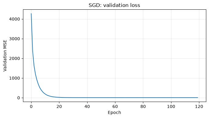
Consider regression by secondary feature $[1,x_1,x_2,x_1^2,x_1x_2,x_2^2]$ and update the coefficient with the gradient of minibatch loss. Because the gradient fluctuates, it manages evaluation losses per epoch unit and data shuffling.

Check with Python

def features(X):
    a, b = X[:, 0], X[:, 1]
    return np.c_[np.ones(len(X)), a, b, a*a, a*b, b*b]

Phi_tr, Phi_te = features(X_train), features(X_test)
mu, sd = y_train.mean(), y_train.std()
yt = (y_train-mu)/sd
w = np.zeros(Phi_tr.shape[1]); lr = 0.03; batch_size = 24
sgd_history = []
for epoch in range(120):
    for idx in rng.permutation(n_train).reshape(-1, batch_size):
        err = Phi_tr[idx] @ w - yt[idx]
        w -= lr * (2/len(idx)) * Phi_tr[idx].T @ err
    pred = (Phi_te @ w)*sd + mu
    sgd_history.append(np.mean((pred-y_test)**2))
print(f"ReceptionRMSE: {np.sqrt(sgd_history[-1]):.2f}")
fig, ax = plt.subplots()
ax.plot(sgd_history)
ax.set_title("SGD: validation loss"); ax.set_xlabel("Epoch"); ax.set_ylabel("Validation MSE")
ax.grid(True, alpha=0.3); plt.tight_layout(); plt.show()

RMSE rating: 2.33

Reading the results

Assessment losses drop significantly from the beginning and then fluctuate slightly. If it stops only at learning loss, overlearning will be overlooked, so evaluation data corresponding to future lots is separated. For time series data, it is more appropriate to design the system of learning from the past and evaluating it in the future rather than random partitioning.

No.096：Adam

Meaning in Practice

If the gradient size differs for each feature, it becomes difficult to adjust with a single learning rate. Adam uses the first and second moments of gradients to adaptively adjust the amount of updates for each coefficient.

Approach to Analysis and Modeling

$m_t=\beta_1m_{t-1}+(1-\beta_1)g_t$, $v_t=\beta_2v_{t-1}+(1-\beta_2)g_t^2$ is biased and updated with $\theta_t=\theta_{t-1}-\eta\hat m_t/(\sqrt{\hat v_t}+\epsilon)$. The default value is the starting point, chosen based on evaluation data.

Check with Python

w_adam = np.zeros(Phi_tr.shape[1]); m = np.zeros_like(w_adam); v = np.zeros_like(w_adam)
beta1, beta2, lr_adam, eps, step = 0.9, 0.999, 0.03, 1e-8, 0
adam_history = []
for epoch in range(120):
    for idx in rng.permutation(n_train).reshape(-1, batch_size):
        step += 1
        err = Phi_tr[idx] @ w_adam - yt[idx]
        g = (2/len(idx)) * Phi_tr[idx].T @ err
        m = beta1*m + (1-beta1)*g; v = beta2*v + (1-beta2)*g*g
        mh, vh = m/(1-beta1**step), v/(1-beta2**step)
        w_adam -= lr_adam*mh/(np.sqrt(vh)+eps)
    pred = (Phi_te @ w_adam)*sd + mu
    adam_history.append(np.mean((pred-y_test)**2))
compare_df = pd.DataFrame({"method": ["SGD", "Adam"],
                           "validation_RMSE": [np.sqrt(sgd_history[-1]), np.sqrt(adam_history[-1])],
                           "best_RMSE": [np.sqrt(min(sgd_history)), np.sqrt(min(adam_history))]})
display(compare_df.round(3))

	method	validation_RMSE	best_RMSE
0	SGD	2.332	2.315
1	Adam	3.078	2.233

Reading the results

Adam can make adjustments easier, but it’s not always better than SGD. Instead of the final epoch, the point at which evaluation loss is minimized is saved, and the data is divided and compared using the same data split and evaluation metrics. Multiple evaluations with random numbers are also necessary.

No.097: Constrained Optimization

Meaning in Practice

Even if losses are minimal, conditions exceeding equipment capacity or safety margins cannot be adopted. Here, in addition to upper and lower limits of temperature and pressure, $x_1+0.8x_2\leq0.35$ representing thermal load are imposed.

Approach to Analysis and Modeling

$\min_x J(x)$ Subject to $g(x)\geq0$ and solved using SLSQP. If the constraint is activation, the optimal point is at the boundary, and sensitivity equivalent to the shadow price leads to value judgments for facility enhancement.

Check with Python

constraint = {"type": "ineq", "fun": lambda x: 0.35 - x[0] - 0.8*x[1],
              "jac": lambda x: np.array([-1.0, -0.8])}
res_con = optimize.minimize(objective, [0, 0], jac=gradient, method="SLSQP",
                            bounds=[(-1.5, 1.5), (-1.5, 1.5)], constraints=[constraint])
unconstrained = np.array([0.8, -0.4])
decision_df = pd.DataFrame([
    ["unconstrained", *unconstrained, objective(unconstrained), 0.35-unconstrained[0]-0.8*unconstrained[1]],
    ["constrained", *res_con.x, res_con.fun, constraint["fun"](res_con.x)]
], columns=["case", "x1", "x2", "loss", "constraint_margin"])
decision_df["temperature_C"] = 210 + 10*decision_df["x1"]
decision_df["pressure_MPa"] = 80 + 10*decision_df["x2"]
display(decision_df.round(3))

	case	x1	x2	loss	constraint_margin	temperature_C	pressure_MPa
0	unconstrained	0.800	-0.400	18.000	-0.13	218.000	76.000
1	constrained	0.733	-0.479	18.451	-0.00	217.334	75.207

Reading the results

Unconstrained solutions break the thermal load constraint, while constrained solutions move within the boundary. Increased losses are the cost of maintaining safety margins. If the constraint margin is almost zero, additional margins for actual operation are set by considering sensor and model errors.

No.098: Automatic Differentiation Library

Meaning in Practice

Manually calculating the differentiation of complex quality models makes it difficult to detect implementation errors. Automatic differentiation applies the chain law to the computational graph, obtaining gradients consistent with the model.

Approach to Analysis and Modeling

Automatic differentiation is not a numerical difference. Records the operations and performs differentiation using backpropagation. Comparing with finite differences is effective for standalone testing, but there are cut-off and rounding errors depending on the notch width.

Check with Python

x_t = torch.tensor([0.2, 0.1], dtype=torch.float64, requires_grad=True)
u, v = x_t[0]-0.8, x_t[1]+0.4
loss_t = 45*u**2 + 30*v**2 + 12*u*v + 18
loss_t.backward()
auto_grad = x_t.grad.detach().numpy()
h = 1e-6; x_np = x_t.detach().numpy()
fd_grad = np.array([(objective(x_np + h*np.eye(2)[j])-objective(x_np - h*np.eye(2)[j]))/(2*h)
                    for j in range(2)])
grad_check = pd.DataFrame({"variable": ["x1", "x2"], "autodiff": auto_grad,
                           "finite_difference": fd_grad, "abs_diff": np.abs(auto_grad-fd_grad)})
display(grad_check)

	variable	autodiff	finite_difference	abs_diff
0	x1	-48.0	-48.0	3.960920e-10
1	x2	22.8	22.8	1.050182e-11

Reading the results

If the automatic differentiation and center difference are close enough, the basic integrity of the gradient implementation can be confirmed. However, matching does not guarantee the validity of the objective function itself. Before learning, gradient checks—including representative points, boundary points, and missing processing—are incorporated into the automated test.

No.099: GPU Numerical Calculation

Meaning in Practice

GPUs can execute large numbers of matrix products in parallel, accelerating image inspection and large-scale learning. On the other hand, for small tabular data, transfer and startup costs dominate, making the CPU more efficient.

Approach to Analysis and Modeling

Evaluation is based not only on computational load but also on total required time, including data transfer, memory capacity, accuracy, reproducibility, and maintenance costs. Here, the available accelerators are determined, and the same matrix product is executed on the selected device. Since velocity values depend on the environment, we use real-data-scale benchmarks for decision-making.

Check with Python

if torch.cuda.is_available():
    device = torch.device("cuda")
elif getattr(torch.backends, "mps", None) and torch.backends.mps.is_available():
    device = torch.device("mps")
else:
    device = torch.device("cpu")

n = 1200
A = torch.randn((n, n), generator=torch.Generator().manual_seed(SEED), dtype=torch.float32).to(device)
B = torch.randn((n, n), generator=torch.Generator().manual_seed(SEED+1), dtype=torch.float32).to(device)
_ = A @ B
if device.type == "cuda": torch.cuda.synchronize()
start = time.perf_counter(); C = A @ B
if device.type == "cuda": torch.cuda.synchronize()
elapsed = time.perf_counter()-start
gpu_check_df = pd.DataFrame({"item": ["selected_device", "matrix_size", "measured_seconds"],
                             "value": [str(device), f"{n} x {n}", f"{elapsed:.4f}"]})
display(gpu_check_df)

	item	value
0	selected_device	mps
1	matrix_size	1200 x 1200
2	measured_seconds	0.0002

Reading the results

The displayed time is a reference value for one run in this environment. Even if the GPU is not selected, the calculation is still normal. In implementation decisions, we measure multiple times after warming up with representative workloads, comparing end-to-end time, costs, and operational personnel from data preparation to result storage.

No.100: Numerical Computation for the Mathematical Laboratory

Meaning in Practice

To turn numerical calculations into value, before algorithm selection, you define decision-making, KPIs, constraints, and verification responsibilities. Finally, create a minimum confirmation table to implement process condition recommendations in production.

Approach to Analysis and Modeling

The recommended criteria are not the “model optimal value,” but rather data coverage, constraint margin, sensitivity, reproducibility, and decision-making candidates who have passed field tests. Compare current condition $x=(0,0)$ and constrained candidates using the same objective function, and list not only improvement rates but also risk countermeasures.

Check with Python

current_x = np.array([0.0, 0.0])
improvement = (objective(current_x)-res_con.fun)/objective(current_x)*100
checklist = pd.DataFrame([
    ["Decision-making", "Total loss of quality, time, and energy", "Defined"],
    ["Data", "Applicable equipment, materials, and seasonal range", "Additional confirmation"],
    ["Numerical Verification", "Convergence, gradient, multiple initials", "Verified"],
    ["restriction", "Set upper and lower limits, heat load, safety margin", "Add extra margin"],
    ["On-site Verification", "Small-scale test→Quality Approval→Phased Expansion", "Before Implementation"],
    ["surveillance", "Input deviation,KPIDegradation and Relearning Conditions", "Before Design"],
], columns=["area", "acceptance_point", "status"])
display(pd.DataFrame({
    "case": ["current", "recommended"],
    "temperature_C": [210, 210+10*res_con.x[0]],
    "pressure_MPa": [80, 80+10*res_con.x[1]],
    "loss": [objective(current_x), res_con.fun]
}).round(2))
print(f"Total loss improvement rate on the model: {improvement:.1f}%")
display(checklist)

	case	temperature_C	pressure_MPa	loss
0	current	210.00	80.00	47.76
1	recommended	217.33	75.21	18.45

Total loss improvement rate on the model: 61.4%

	area	acceptance_point	status
0	Decision-making	Total loss of quality, time, and energy	Defined
1	Data	Applicable equipment, materials, and seasonal range	Additional confirmation
2	Numerical Verification	Convergence, gradient, multiple initials	Verified
3	restriction	Set upper and lower limits, heat load, safety margin	Add extra margin
4	On-site Verification	Small-scale test→Quality Approval→Phased Expansion	Before Implementation
5	surveillance	Input deviation,KPIDegradation and Relearning Conditions	Before Design

Reading the results

While the model suggests there is room for improvement in total loss compared to current conditions, this does not guarantee actual performance. Additional confirmation, Before Implementation, and Before Design are resolved before becoming a candidate for implementation. In Numerical Computation Support at the Mathematical Laboratory, we handle constraint organization, acceptance testing, and monitoring design at the same weight as model creation.

Practical Implications Seen Through Target Exercise

1. Agree on the objective function before optimization: Not only defect rates, but also time, energy, waste, and equipment load are organized into the same unit as decision-making.
2. Fast methods are not always better: Depending on the data volume, number of variables, curvature, memory, and constraints, choose gradient descent, quasi-Newton, or mini-batch methods.
3. No Restrictions Added Afterwards: Equipment limits, safety, quality assurance, and changeable ranges are clearly indicated in the optimization problems, ensuring margin for measurement errors.
4. Distinguishing calculation results from actual process effects: The improvement rate on the model is hypothetical. Phase tests and evaluation periods are set to confirm causal effects.
5. GPUis not the goal: Measure model size and latency bottlenecks, and select based on total cost and maintainability.

What is necessary for practical implementation

• Target KPIs, Currency Conversion Rules, Responsible Departments, and Approvals
• Confirmation of data quality and applicable scope across materials, molds, equipment, and seasons
• Documentation of hardware and soft constraints, safety margins, and recovery conditions during abnormalities
• Design of baselines, evaluation metrics, holdout periods, and stage trials
• Version management of code, dependency libraries, random numbers, models, and input data
• Continuous monitoring of input distribution deviations, forecast errors, KPIs, and constraint margins

Conclusion

From No.091 to No.100, we connected the gradient descent method to GPU numerical calculations to optimization of hypothetical process conditions. What matters is not whether advanced methods were used, but the ability to explain objective functions and constraints, verify with unknown data, and enable safe approval and shutdown on site. Check numerical behavior with small proxy problems, and in actual processes, limit the scope of application and introduce it step by step.

Consultations for Corporations

At Mathematical Laboratory, we support decision-making in manufacturing processes from quality forecasting, process condition optimization, mathematical model validation, PoC design, to operational monitoring. You can consult with us from the stage where you may have a predictive model but it does not lead to recommended conditions, if you want to design optimizations with constraints, or if you want to evaluate the computing infrastructure including the CPU/GPU.

📩 Contact Us: surikobo.co.jp/contact Please feel free to consult us first.