Predicting the Time Variations of Heating, Reaction, and Transport: Ten Exercises of Ordinary Differential Equations Useful for Manufacturing Decision-Making (No.071–No.080)

In this article, we connect representative numerical solutions to ordinary differential equations (ODE) to Design of heat treatment conditions, quality prediction of reaction tanks, equipment vibration, infection and absenteeism risks, furnace operation planning at a fictional precision parts factory. The goal is not to memorize calculation formulas, but to distinguish calculation accuracy, computation time, model validity, and design simulations that can be used to determine operating conditions.

The scope of coverage includes No.071 to No.080 (Euler method, modified Euler method, Runge–Kutta method, adaptive notch width method, stiffness equations, Adams method, BDF method, pendulum, SIR model, physical simulation). All listed data and parameters are hypothetical values for explanatory purposes.

[!NOTE] This material is a notebook previously used by Surikoubo (or personally by the representative, Kazuyama), and has been reconstructed, edited, and published with the company’s permission.
All data listed is fictional and has no relation whatsoever to real companies, factories, or figures.

Introduction: Practical Challenges in Manufacturing Covered in This Article

In manufacturing sites, temperature, concentration, pressure, vibration, and inventory all change over time. It is necessary to know not only the “current value” but also the When to enter the standard range, how far it goes too far, and how many minutes of buffer time is left during abnormalities. when the input amount and outside temperature change. In this article, we will discuss the rate of change of state $y(t)$

$\frac{dy}{dt}=f(t,y;\theta),\qquad y(t_0)=y_0$

and then calculate the future trajectory using numerical integration. $\theta$ are model parameters such as heat capacity and reaction rate.

Common situations on site

• Estimate the time when the heat treatment tank will reach the target temperature and decide the production start time.
• Fast and slow reactions are mixed, and under normal calculations, the notch width must be extremely small
• We want to calibrate the model from the time-series data of existing equipment and pre-evaluate the impact of condition changes.
• Even if the calculation results are smooth, it is impossible to determine whether it is a numerical error or a model error.

Why is this issue so difficult to judge?

The discretized calculated values have Cancellation error and rounding errors depending on the notch width. On the other hand, differences from actual equipment include parameter estimation errors, unmeasured disturbances, and deficiencies in model structure. Simply switching to a higher-level solution does not necessarily mean the actual equipment prediction will be correct. Both convergence confirmation by halving the increment width and validation using independent measured data are required.

Overview of Exercise covered this time

In the first half, we solve the same cooling model using multiple methods and compare accuracy and computational complexity. In the middle section, we will handle rigid reaction systems and multi-stage methods. In the second half, we will examine the entire process from modeling to decision-making, using pendulums, SIR models, and two-region heating furnaces as subjects.

Preparing the Python environment

NumPy performs array calculations, pandas tables, SciPy verified ODE solvers, and matplotlib visualizations. Fix the random number seed so you can reproduce the same result.

%matplotlib inline
import platform
import numpy as np
import pandas as pd
import matplotlib
import matplotlib.pyplot as plt
from scipy.integrate import solve_ivp

SEED = 20260712
rng = np.random.default_rng(SEED)
pd.set_option("display.precision", 4)
print(f"Python: {platform.python_version()}")
print(f"NumPy: {np.__version__}, pandas: {pd.__version__}")
print(f"matplotlib: {matplotlib.__version__}")

Python: 3.13.1
NumPy: 2.5.1, pandas: 3.0.3
matplotlib: 3.11.0

Creation of Fictional Data

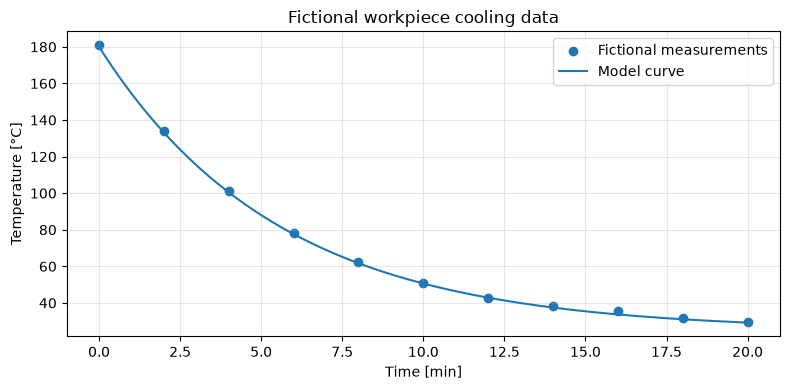
For the initial comparison, we use Newton’s cooling law, which represents the cooling of parts taken out of the furnace. For $T$ component temperature, $T_a$ ambient temperature, and $k$ cooling coefficient,

$\frac{dT}{dt}=-k(T-T_a),\qquad T(t)=T_a+(T_0-T_a)e^{-kt}$

That’s right. In the latter half, we separately define fictitious parameters such as reaction concentration, pendulum, absenteeism risk, and the two in-furnace regions. Analytical solutions are used only as a standard to measure errors in numerical solutions.

T0, T_ambient, k_cool = 180.0, 25.0, 0.18

def cooling_rhs(t, y):
    return np.asarray([-k_cool * (y[0] - T_ambient)])

def cooling_exact(t):
    return T_ambient + (T0 - T_ambient) * np.exp(-k_cool * np.asarray(t))

base_times = np.arange(0, 21, 2)
fictional_measurements = cooling_exact(base_times) + rng.normal(0, 1.2, len(base_times))
cooling_data = pd.DataFrame({"time_min": base_times, "measured_temp_C": fictional_measurements})
display(cooling_data.head())

plt.figure(figsize=(8, 4))
plt.scatter(base_times, fictional_measurements, label="Fictional measurements")
tt = np.linspace(0, 20, 200)
plt.plot(tt, cooling_exact(tt), label="Model curve")
plt.title("Fictional workpiece cooling data")
plt.xlabel("Time [min]"); plt.ylabel("Temperature [°C]")
plt.grid(True, alpha=0.3); plt.legend(); plt.tight_layout(); plt.show()

	time_min	measured_temp_C
0	0	180.8863
1	2	133.9578
2	4	100.9478
3	6	78.1300
4	8	62.2210

No.071: Euler’s Method

Meaning in Practice

The Euler method assumes that the current rate of change will continue for a short period and predicts the following state. It is easy to use for simple PLC predictions and model concept validation, and serves as a starting point for understanding how the increment width affects judgment outcomes.

Approach to Analysis and Modeling

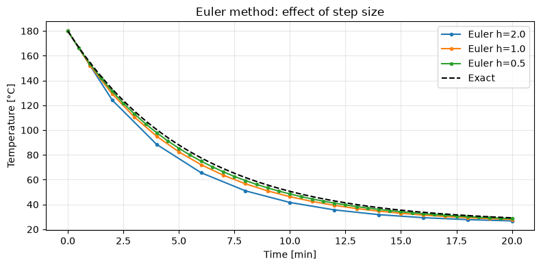
If the notch width is $h$, it is $y_{n+1}=y_n+h f(t_n,y_n)$. The local error in step 1 is $O(h^2)$, and the global error after advancing a certain section is $O(h)$. Therefore, if you cut the notch width in half, the error will roughly halve within a sufficiently small range.

Check with Python

def euler(f, t0, tf, y0, h):
    t = np.arange(t0, tf + h/2, h)
    y = np.empty((len(t), len(np.atleast_1d(y0))))
    y[0] = np.atleast_1d(y0)
    for n in range(len(t) - 1):
        y[n+1] = y[n] + h * f(t[n], y[n])
    return t, y

rows = []
plt.figure(figsize=(8, 4))
for h in [2.0, 1.0, 0.5]:
    t_e, y_e = euler(cooling_rhs, 0, 20, [T0], h)
    err = abs(y_e[-1, 0] - cooling_exact(20))
    rows.append({"step_min": h, "T_at_20_C": y_e[-1, 0], "abs_error_C": err})
    plt.plot(t_e, y_e[:, 0], marker="o", ms=3, label=f"Euler h={h}")
plt.plot(tt, cooling_exact(tt), "k--", label="Exact")
display(pd.DataFrame(rows))
plt.title("Euler method: effect of step size")
plt.xlabel("Time [min]"); plt.ylabel("Temperature [°C]")
plt.grid(True, alpha=0.3); plt.legend(); plt.tight_layout(); plt.show()

	step_min	T_at_20_C	abs_error_C
0	2.0	26.7870	2.4481
1	1.0	27.9283	1.3069
2	0.5	28.5644	0.6708

Reading the results

Reducing the notch width reduces the error after 20 minutes. Even with rough cuts, curves appear smooth, so don’t rely solely on appearance. For example, when determining “transport is possible below 60°C,” the temperature error is converted into a time margin, and the safety tolerance is determined first.

No.072: Modified Euler Method

Meaning in Practice

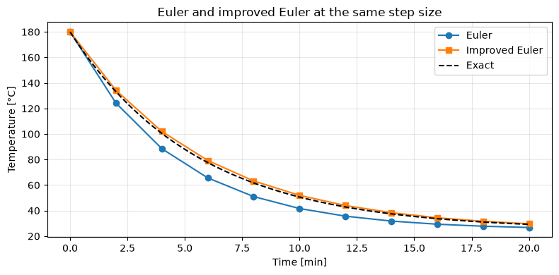
If the heating and cooling rates change within a section, only the slope of the section start point will cause bias. The Modified Euler Method (Heun method) averages the slope of the start and predicted endpoints, improving accuracy with minimal additional calculations.

Approach to Analysis and Modeling

Create a prediction value $\tilde y_{n+1}=y_n+h f(t_n,y_n)$,

$y_{n+1}=y_n+\frac{h}{2}\{f(t_n,y_n)+f(t_{n+1},\tilde y_{n+1})\}$

I will correct it accordingly. The global error is $O(h^2)$. Compare with the Euler method at the same increment and quantify the effect of the method change.

Check with Python

def heun(f, t0, tf, y0, h):
    t = np.arange(t0, tf + h/2, h)
    y = np.empty((len(t), len(np.atleast_1d(y0)))); y[0] = y0
    for n in range(len(t)-1):
        k1 = f(t[n], y[n])
        predictor = y[n] + h * k1
        k2 = f(t[n+1], predictor)
        y[n+1] = y[n] + h * (k1 + k2) / 2
    return t, y

h = 2.0
t_e, y_e = euler(cooling_rhs, 0, 20, [T0], h)
t_h, y_h = heun(cooling_rhs, 0, 20, [T0], h)
compare = pd.DataFrame({
    "method": ["Euler", "Improved Euler"],
    "T_at_20_C": [y_e[-1, 0], y_h[-1, 0]],
    "abs_error_C": [abs(y_e[-1, 0]-cooling_exact(20)), abs(y_h[-1, 0]-cooling_exact(20))]
})
display(compare)
plt.figure(figsize=(8, 4))
plt.plot(t_e, y_e[:, 0], "o-", label="Euler")
plt.plot(t_h, y_h[:, 0], "s-", label="Improved Euler")
plt.plot(tt, cooling_exact(tt), "k--", label="Exact")
plt.title("Euler and improved Euler at the same step size")
plt.xlabel("Time [min]"); plt.ylabel("Temperature [°C]")
plt.grid(True, alpha=0.3); plt.legend(); plt.tight_layout(); plt.show()

	method	T_at_20_C	abs_error_C
0	Euler	26.787	2.4481
1	Improved Euler	29.688	0.4529

Reading the results

Even at the same 2-minute increments, the error of the modified Euler method is significantly reduced. However, the function is evaluated twice per step. In embedded control, the allowable error, computation time, and control cycle cutoff are listed to determine the method.

No.073: Runge–Kutta Method

Meaning in Practice

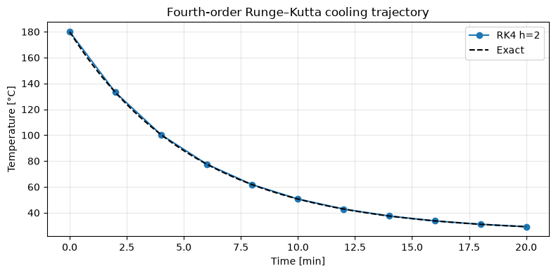
The 4th order Runge–Kutta method (RK4) is a fixed chopping method widely used in thermal, reaction, and motion models. Slope is evaluated at multiple points within a single step, making it easier to obtain the accuracy needed for comparing driving conditions.

Approach to Analysis and Modeling

$k_1=f(t_n,y_n)$, $k_2=f(t_n+h/2,y_n+hk_1/2)$, $k_3=f(t_n+h/2,y_n+hk_2/2)$, $k_4=f(t_n+h,y_n+hk_3)$,

$y_{n+1}=y_n+\frac{h}{6}(k_1+2k_2+2k_3+k_4)$

Let’s say so. The global error is $O(h^4)$, but stability is not guaranteed unconditionally.

Check with Python

def rk4(f, t0, tf, y0, h):
    t = np.arange(t0, tf + h/2, h)
    y = np.empty((len(t), len(np.atleast_1d(y0)))); y[0] = y0
    for n in range(len(t)-1):
        k1 = f(t[n], y[n]); k2 = f(t[n]+h/2, y[n]+h*k1/2)
        k3 = f(t[n]+h/2, y[n]+h*k2/2); k4 = f(t[n]+h, y[n]+h*k3)
        y[n+1] = y[n] + h*(k1+2*k2+2*k3+k4)/6
    return t, y

method_rows = []
for name, solver, evaluations in [("Euler", euler, 1), ("Improved Euler", heun, 2), ("RK4", rk4, 4)]:
    t_m, y_m = solver(cooling_rhs, 0, 20, [T0], 2.0)
    method_rows.append({"method": name, "rhs_calls_per_step": evaluations,
                        "abs_error_at_20_C": abs(y_m[-1,0]-cooling_exact(20))})
display(pd.DataFrame(method_rows))

t_r, y_r = rk4(cooling_rhs, 0, 20, [T0], 2.0)
plt.figure(figsize=(8, 4))
plt.plot(t_r, y_r[:, 0], "o-", label="RK4 h=2")
plt.plot(tt, cooling_exact(tt), "k--", label="Exact")
plt.title("Fourth-order Runge–Kutta cooling trajectory")
plt.xlabel("Time [min]"); plt.ylabel("Temperature [°C]")
plt.grid(True, alpha=0.3); plt.legend(); plt.tight_layout(); plt.show()

	method	rhs_calls_per_step	abs_error_at_20_C
0	Euler	1	2.4481
1	Improved Euler	2	0.4529
2	RK4	4	0.0029

Reading the results

RK4 shows even smaller errors with the same notch width. A simple model is a sufficient option, but when input changes suddenly or just before safety judgments, the output points are finely tuned. Even in higher-order methods, one step crossing discontinuous control inputs needs to be split.

No.074: Adaptive Notch Width Method

Meaning in Practice

Immediately after the furnace is set up, temperature changes are rapid, and near steady-state temperature, it slows down. Instead of engraving the entire section finely, if the engraving width is reduced only for the sections with large errors, both accuracy and calculation time can be achieved.

Approach to Analysis and Modeling

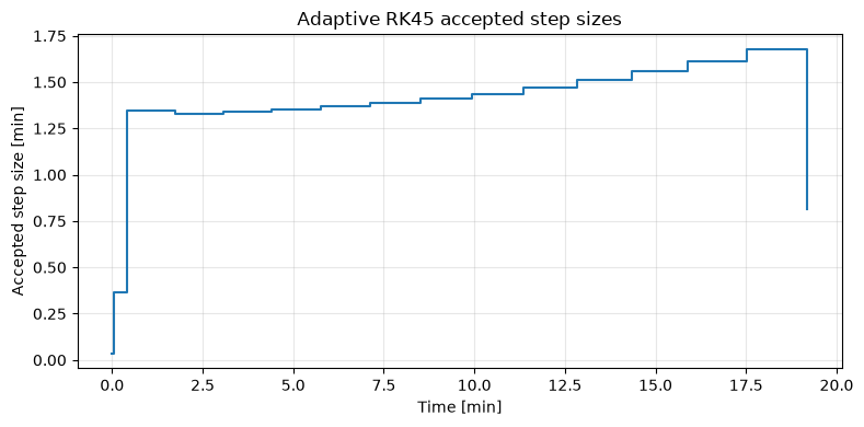
The embedded Runge–Kutta method estimates local errors from approximate differences of different degrees. rtol is the allowable error proportional to the size of the state, and atol is the absolute allowable error near zero. The tolerance scale is determined based on the thermometer’s accuracy and judgment margin.

Check with Python

adaptive_rows = []
solutions = {}
for rtol in [1e-3, 1e-6, 1e-9]:
    sol = solve_ivp(cooling_rhs, (0, 20), [T0], method="RK45", rtol=rtol, atol=rtol*0.1)
    solutions[rtol] = sol
    adaptive_rows.append({"rtol": rtol, "accepted_points": len(sol.t), "rhs_calls": sol.nfev,
                          "abs_error_at_20_C": abs(sol.y[0,-1]-cooling_exact(20))})
display(pd.DataFrame(adaptive_rows))
sol = solutions[1e-6]
steps = np.diff(sol.t)
plt.figure(figsize=(8, 4))
plt.step(sol.t[:-1], steps, where="post")
plt.title("Adaptive RK45 accepted step sizes")
plt.xlabel("Time [min]"); plt.ylabel("Accepted step size [min]")
plt.grid(True, alpha=0.3); plt.tight_layout(); plt.show()

	rtol	accepted_points	rhs_calls	abs_error_at_20_C
0	1.0000e-03	7	38	1.0039e-02
1	1.0000e-06	17	98	8.0528e-06
2	1.0000e-09	56	332	8.0192e-09

Reading the results

Tightening the tolerance increases the number of function evaluations and reduces endpoint error. The internal time received by the solver and the output time required for reporting and control are different things. Quality judgment times are clearly indicated in t_eval or event detection, and only the number of internal steps is not used as a KPI.

No.075: Rigid Equations

Meaning in Practice

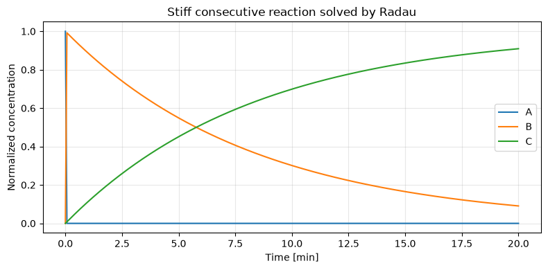
In cleaning and catalytic reactions, components that are nearly instantaneous coexist with slower components that control manufacturing time. In such rigid systems, the explicit method requires minimal increments for stability rather than precision.

Approach to Analysis and Modeling

The imaginary continuous reaction $A\to B\to C$

$A'=-k_1A,\quad B'=k_1A-k_2B,\quad C'=k_2B$

Let’s say so. $k_1\gg k_2$ time scales differ significantly. Compare the positive RK method and the negative Radau method for rigidity with the same tolerance margin.

Check with Python

k1, k2 = 1000.0, 0.12
def stiff_reaction(t, y):
    A, B, C = y
    return [-k1*A, k1*A-k2*B, k2*B]

stiff_rows = []
stiff_solutions = {}
for method in ["RK45", "Radau"]:
    sol_s = solve_ivp(stiff_reaction, (0, 20), [1, 0, 0], method=method,
                      rtol=1e-6, atol=1e-9, dense_output=True)
    stiff_solutions[method] = sol_s
    stiff_rows.append({"method": method, "rhs_calls": sol_s.nfev,
                       "accepted_points": len(sol_s.t), "mass_balance_error": abs(sol_s.y[:,-1].sum()-1)})
display(pd.DataFrame(stiff_rows))
t_plot = np.linspace(0, 20, 300)
ys = stiff_solutions["Radau"].sol(t_plot)
plt.figure(figsize=(8, 4))
for i, label in enumerate(["A", "B", "C"]): plt.plot(t_plot, ys[i], label=label)
plt.title("Stiff consecutive reaction solved by Radau")
plt.xlabel("Time [min]"); plt.ylabel("Normalized concentration")
plt.grid(True, alpha=0.3); plt.legend(); plt.tight_layout(); plt.show()

	method	rhs_calls	accepted_points	mass_balance_error
0	RK45	42542	6087	1.1102e-15
1	Radau	949	135	7.6688e-09

Reading the results

Even under the same precision conditions, positive RK45 is constrained by fast reactions and requires numerous functional evaluations. While implicit solutions like Radau require one step heavier, rigid systems reduce the overall computational complexity. Whether the total concentration is maintained at 1 or that no negative concentration is observed is also included in the acceptance test.

No.076: Adams Method

Meaning in Practice

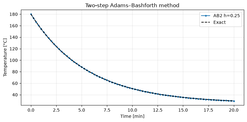
In continuous operation, where model evaluation is expensive and conditions change smoothly, multi-stage methods that reuse past tilt are effective. Here, the two-step Adams–Bashforth method (AB2) limits each step to a single new assessment.

Approach to Analysis and Modeling

$y_{n+1}=y_n+h\left(\frac32f_n-\frac12f_{n-1}\right)$

is a positive two-step method. The first point needs to be made using a different method, and here we will use RK4 in just one step. Because it uses historical information, handling step width changes and discontinuous input is more complex than the single-step method.

Check with Python

def adams_bashforth2(f, t0, tf, y0, h):
    t = np.arange(t0, tf+h/2, h)
    y = np.empty((len(t), len(np.atleast_1d(y0)))); y[0] = y0
    k1 = f(t[0], y[0]); k2 = f(t[0]+h/2, y[0]+h*k1/2)
    k3 = f(t[0]+h/2, y[0]+h*k2/2); k4 = f(t[0]+h, y[0]+h*k3)
    y[1] = y[0] + h*(k1+2*k2+2*k3+k4)/6
    f_prev, f_now = f(t[0], y[0]), f(t[1], y[1])
    for n in range(1, len(t)-1):
        y[n+1] = y[n] + h*(1.5*f_now-0.5*f_prev)
        f_prev, f_now = f_now, f(t[n+1], y[n+1])
    return t, y

ab_rows = []
for h in [1.0, 0.5, 0.25]:
    t_ab, y_ab = adams_bashforth2(cooling_rhs, 0, 20, [T0], h)
    ab_rows.append({"step_min": h, "steps": len(t_ab)-1,
                    "abs_error_at_20_C": abs(y_ab[-1,0]-cooling_exact(20))})
display(pd.DataFrame(ab_rows))
plt.figure(figsize=(8, 4))
plt.plot(t_ab, y_ab[:,0], "o-", ms=3, label="AB2 h=0.25")
plt.plot(tt, cooling_exact(tt), "k--", label="Exact")
plt.title("Two-step Adams–Bashforth method")
plt.xlabel("Time [min]"); plt.ylabel("Temperature [°C]")
plt.grid(True, alpha=0.3); plt.legend(); plt.tight_layout(); plt.show()

	step_min	steps	abs_error_at_20_C
0	1.00	20	0.2181
1	0.50	40	0.0530
2	0.25	80	0.0131

Reading the results

When the notch width is halved, the error approaches roughly one-quarter in sufficiently small areas, allowing secondary accuracy to be confirmed. AB2 is designed for smooth, non-rigid problems. When equipment is turned on or off or material input times, the history is reinitialized, and past slopes are not extrapolated across discontinuity points.

No.077: BDF Method

Meaning in Practice

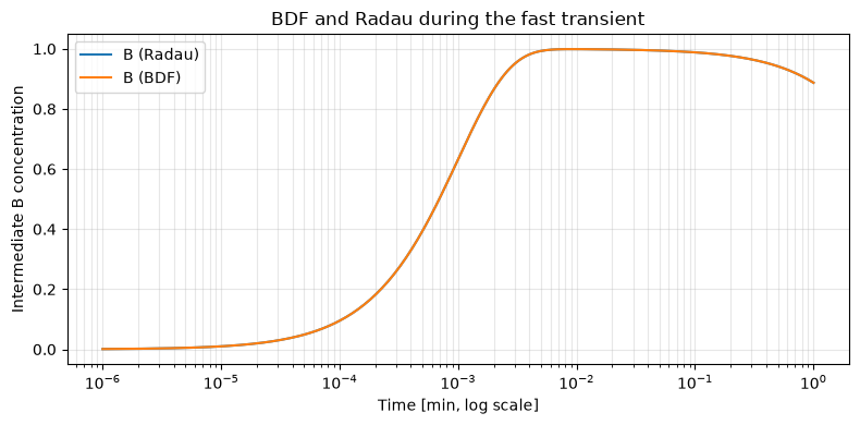
BDF (Backward Difference Formula) is a multi-stage implicit method used in rigid reaction and heat balance models. If a long steady operation involves rapid transience, progress is made while ensuring stability.

Approach to Analysis and Modeling

The primary BDF (Backward Euler method) is

$y_{n+1}=y_n+h f(t_{n+1},y_{n+1})$

And the unknown $y_{n+1}$ also appears on the right side. At each step, you need to solve the nonlinear equation. In practice, we do not build our own but use verified implementations with error control, order changes, and Jacobian processing.

Check with Python

bdf_rows = []
bdf_solutions = {}
for method in ["Radau", "BDF"]:
    sol_b = solve_ivp(stiff_reaction, (0, 20), [1, 0, 0], method=method,
                      rtol=1e-6, atol=1e-9, dense_output=True)
    bdf_solutions[method] = sol_b
    bdf_rows.append({"method": method, "rhs_calls": sol_b.nfev, "jacobian_evals": sol_b.njev,
                     "lu_decompositions": sol_b.nlu, "final_C": sol_b.y[2,-1]})
display(pd.DataFrame(bdf_rows))
t_zoom = np.geomspace(1e-6, 1, 240)
plt.figure(figsize=(8, 4))
for method in ["Radau", "BDF"]:
    plt.semilogx(t_zoom, bdf_solutions[method].sol(t_zoom)[1], label=f"B ({method})")
plt.title("BDF and Radau during the fast transient")
plt.xlabel("Time [min, log scale]"); plt.ylabel("Intermediate B concentration")
plt.grid(True, which="both", alpha=0.3); plt.legend(); plt.tight_layout(); plt.show()

	method	rhs_calls	jacobian_evals	lu_decompositions	final_C
0	Radau	949	3	62	0.9093
1	BDF	385	1	38	0.9093

Reading the results

The fact that BDF and Radau return nearly identical concentration orbitals is a strong mutual confirmation. However, matching does not prove the model’s correctness. In addition to comparison with actual measurements, we conduct sensitivity analyses with varying reaction rates, confirm the substance balance, and non-negativity, and evaluate the shortening of calculations when providing Jacobian data.

No.078: Pendulum Simulation

Meaning in Practice

The sway of the transport arm and the lifting load affects stopping accuracy, cycle time, and safety margin. The pendulum is a basic example of converting the second-floor equation of motion into the first-floor coordinated ODE, leading to the evaluation of residual vibration in equipment.

Approach to Analysis and Modeling

For $\theta$ angle, $\omega$ angular velocity, $L$ length, and $c$ damping,

$\theta'=\omega,\qquad \omega'=-\frac{g}{L}\sin\theta-c\omega$

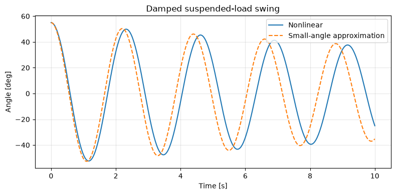
Let’s say so. Since small-angle approximation $\sin\theta\approx\theta$ increases error with large amplitudes, check the difference with nonlinear models.

Check with Python

g, L, damping = 9.81, 1.2, 0.08
def pendulum(t, y): return [y[1], -(g/L)*np.sin(y[0])-damping*y[1]]
def pendulum_linear(t, y): return [y[1], -(g/L)*y[0]-damping*y[1]]

t_eval = np.linspace(0, 10, 501)
y0_p = [np.deg2rad(55), 0]
sol_nl = solve_ivp(pendulum, (0,10), y0_p, t_eval=t_eval, rtol=1e-9, atol=1e-11)
sol_li = solve_ivp(pendulum_linear, (0,10), y0_p, t_eval=t_eval, rtol=1e-9, atol=1e-11)
angle_diff = np.max(np.abs(np.rad2deg(sol_nl.y[0]-sol_li.y[0])))
print(f"Maximum angle difference from small-angle model: {angle_diff:.2f} deg")
plt.figure(figsize=(8, 4))
plt.plot(t_eval, np.rad2deg(sol_nl.y[0]), label="Nonlinear")
plt.plot(t_eval, np.rad2deg(sol_li.y[0]), "--", label="Small-angle approximation")
plt.title("Damped suspended-load swing")
plt.xlabel("Time [s]"); plt.ylabel("Angle [deg]")
plt.grid(True, alpha=0.3); plt.legend(); plt.tight_layout(); plt.show()

Maximum angle difference from small-angle model: 38.59 deg

Reading the results

At an initial angle of 55 degrees, the phase difference with the small-angle approximation accumulates. Nonlinear models should be used for stop wait times and interference checks. When introducing into actual equipment, the hanging length, friction, and travel acceleration are identified, and the maximum angle and setting time are verified according to load conditions.

No.079: SIR Model

Meaning in Practice

Absenteeism due to the pandemic affects staffing and delivery risks. The SIR model is not a diagnostic tool but a simplified model used for scenario comparison of contact suppression and cheering staff preparation.

Approach to Analysis and Modeling

Workers are divided into sensitive $S$, infected $I$, and recovering $R$,

$S'=-\beta SI/N,\quad I'=\beta SI/N-\gamma I,\quad R'=\gamma I$

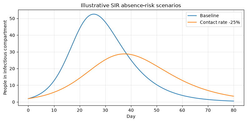
Let’s say so. The simple indicator of the basic reproduction number is $R_0=\beta/\gamma$. Here, we compare it to a scenario where the contact rate is reduced by 25%.

Check with Python

N, gamma = 240, 1/7
def sir_rhs(beta):
    def rhs(t, y):
        S, I, R = y
        return [-beta*S*I/N, beta*S*I/N-gamma*I, gamma*I]
    return rhs

sir_rows = []
plt.figure(figsize=(8, 4))
days = np.linspace(0, 80, 321)
for label, beta in [("Baseline", 0.34), ("Contact rate -25%", 0.34*0.75)]:
    sol_sir = solve_ivp(sir_rhs(beta), (0,80), [238,2,0], t_eval=days, rtol=1e-8, atol=1e-10)
    peak_idx = np.argmax(sol_sir.y[1])
    sir_rows.append({"scenario": label, "R0": beta/gamma,
                     "peak_absent_people": sol_sir.y[1,peak_idx], "peak_day": days[peak_idx]})
    plt.plot(days, sol_sir.y[1], label=label)
display(pd.DataFrame(sir_rows))
plt.title("Illustrative SIR absence-risk scenarios")
plt.xlabel("Day"); plt.ylabel("People in infectious compartment")
plt.grid(True, alpha=0.3); plt.legend(); plt.tight_layout(); plt.show()

	scenario	R0	peak_absent_people	peak_day
0	Baseline	2.380	52.5647	25.5
1	Contact rate -25%	1.785	28.7663	37.5

Reading the results

Assuming a lower contact rate, the number of people at peak would decrease, and the peak period would change. This is not a definitive measure of the effectiveness of the measures, but rather a comparison of the amount of support personnel and work-in-progress inventory prepared. In practice, personal information is aggregated, public guidance is prioritized, and factors omitted such as interdepartmental contact, concealment, testing, and vaccination are clearly stated.

No.080: Physical Simulation

Meaning in Practice

If the temperature inside the furnace is considered uniform, there is a quality risk where the core of the component remains unheated even if the surface sensor reaches the target. Using a two-domain centralized constant model, we compare the heating time and temperature difference for each heater output candidate.

Approach to Analysis and Modeling

The energy balance between the furnace air temperature $T_a$ and the core temperature of the parts $T_c$

$C_aT_a'=P-h_a(T_a-T_{env})-h_c(T_a-T_c),\qquad C_cT_c'=h_c(T_a-T_c)$

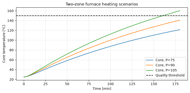
Let’s say so. Change the input $P$ to set the time when the core temperature reaches the lower quality limit and the maximum temperature difference as KPIs.

Check with Python

C_air, C_core, h_loss, h_core, T_env = 18.0, 65.0, 0.45, 2.8, 25.0
def furnace_rhs(power):
    def rhs(t, y):
        T_air, T_core = y
        return [(power-h_loss*(T_air-T_env)-h_core*(T_air-T_core))/C_air,
                h_core*(T_air-T_core)/C_core]
    return rhs

minutes = np.linspace(0, 180, 721)
furnace_rows = []
plt.figure(figsize=(8, 4))
for power in [75.0, 90.0, 105.0]:
    sf = solve_ivp(furnace_rhs(power), (0,180), [25,25], t_eval=minutes, method="RK45",
                   rtol=1e-7, atol=1e-9)
    reached = np.flatnonzero(sf.y[1] >= 150)
    reach_time = minutes[reached[0]] if len(reached) else np.nan
    furnace_rows.append({"power_kJ_per_min": power, "core_150C_time_min": reach_time,
                         "max_air_core_gap_C": np.max(sf.y[0]-sf.y[1]), "core_at_180_C": sf.y[1,-1]})
    plt.plot(minutes, sf.y[1], label=f"Core, P={power:.0f}")
display(pd.DataFrame(furnace_rows))
plt.axhline(150, color="k", ls="--", label="Quality threshold")
plt.title("Two-zone furnace heating scenarios")
plt.xlabel("Time [min]"); plt.ylabel("Core temperature [°C]")
plt.grid(True, alpha=0.3); plt.legend(); plt.tight_layout(); plt.show()

	power_kJ_per_min	core_150C_time_min	max_air_core_gap_C	core_at_180_C
0	75.0	NaN	17.4573	121.3896
1	90.0	NaN	20.9487	140.6676
2	105.0	160.5	24.4402	159.9455

Reading the results

Increasing output accelerates the reach of the 150°C core temperature, but you should also check the maximum temperature difference between the air and the center. Capacity enhancement is determined not only by time to arrive, but also through multi-purpose evaluations including surface overheating, energy intensity, temperature uniformity, and equipment limits. This dual-domain model is used for narrowing down candidates, and the selection criteria are confirmed through actual machine testing.

Practical Implications Seen Through Target Exercise

1. Choosing Solution Methods Based on Purpose and Time Scale: For concept verification, the Euler method is recommended; for smooth non-rigid problems, the RK method is recommended; and for systems with mixed fast and slow phenomena, Radau or BDF are candidates.
2. Setting the tolerance for error per business unit:rtol=1e-6 is not chosen out of convention, but rather linked to a range of judgments such as “temperature ± 0.5°C” or “arrival time ± 1 minute.”
3. Distinguishing numerical errors from model errors: Numerical errors are checked by increment convergence, and model errors are evaluated through actual measurements of different lots and conditions.
4. Testing Conservation Laws and Physical Constraints: Material balance, energy balance, non-negative concentration, and upper and lower limits of equipment are stronger verification materials than they appear on the graph.
5. Simulation is a tool for comparison.: Instead of making a single prediction, set conditions and parameters to indicate the boundary where decisions change.

What is necessary for practical implementation

• Purpose/KPIagreement: Define which to optimize in quality judgment, cycle time, energy, or safety margin.
• Data Design: Time synchronization, sensor calibration, and storage of input, disturbance, equipment status, and lot information
• Parameter Identification and Validation Segmentation: Separate the operational data used for calibration from the performance evaluation data
• Uncertainty and Sensitivity Analysis: Adjust heat capacity, reaction speed, initial state, and confirm the conditions under which the conclusion is reversed.
• Solver acceptance test: Automatically tests tolerance errors, conservation rules, abnormal inputs, event times, and reproducibility
• Operations Design: Record model versions, parameters, inputs, execution times, results, and approvers, creating a system that allows human intervention.
• Phased Implementation: Connecting to control and planning through past data reproduction, shadow operations, and trials in limited processes.

Conclusion

Numerical methods for ordinary differential equations transform manufacturing phenomena with time changes into comparable forms such as “what happens if conditions are changed.” The differences from the Euler method, RK method, adaptive scale, multi-stage method, and rigidity-oriented solutions lie not only in accuracy but also in stability and computational cost. Practical value is not generated by advanced solvers alone, but when a reasonable income and expenditure model, on-site tolerance tolerance, measurement verification, and decision-making processes are all designed in an integrated manner.

Consultations for Corporations

At Mathematical Laboratory, we support the construction of simulations for heat, reactions, and facility motion, parameter identification using measured data, verification of calculation accuracy, and design from PoC to operation. You can consult with us from the stage where you want to transfer existing Excel calculations to verifiable models or explore conditions while reducing the number of experiments.

📩 Contact Us: surikobo.co.jp/contact
Please feel free to consult us first.