Deciphering Equipment Vibration and Process Networks through ‘Eigenvalues’: 10 Numerical Calculations Effective for Manufacturing Decision-Making (No.041–No.050)

This article connects eigenvalue problems, iterative methods, matrix decomposition, and graph analysis to Equipment maintenance, sensor monitoring, and process improvement in a fictional precision parts factory. The goal is not to calculate formulas themselves, but to determine which variation to prioritize, what to approximate with large-scale data, and which steps are most prone to downtime risks.

[!NOTE] This material is a notebook previously used by Surikoubo (or personally by the representative, Kazuyama), and has been reconstructed, edited, and published with the company’s permission.
All data listed is fictional and has no relation whatsoever to real companies, factories, or figures.

Introduction: Practical Challenges in Manufacturing Covered in This Article

At the target factory, vibration sensors across multiple equipment fluctuate in correlation, and information on work-in-progress, reprocessing, and inspection circulates between processes. Relying solely on individual averages or upper limits can overlook abnormal modes common to equipment groups and critical processes throughout the network. In this article, we will extract the “main directions” of the queue and consider where to direct the finite maintenance man-hours.

Common situations on site

• The number of sensors is increasing, but only the number of alarms is rising.
• Correlated vibrations are monitored at individual thresholds for each facility
• All eigenvalues are calculated precisely, but only the top few are used for decision-making
• Although there is a process chart, it has not been able to evaluate the overall impact, including reprocessing loops and information dependence.

Why is this issue so difficult to judge?

Each element of a matrix is a local relationship, but eigenvalues and eigenvectors represent the repeated propagation of the relationship. On the other hand, the larger the matrix, the more trade-offs arise between accuracy, computation time, and memory. Furthermore, mathematically large components do not directly imply causality or investment returns. It is necessary to interpret site knowledge, data quality, and downtime losses together.

Overview of Exercise covered this time

No.	Theme	Judgment in the manufacturing industry
041	What is the eigenvalue problem?	Identifying Dominant Facility Changes
042	Exponentiation	High-speed estimation of maximum variation modes
043	reverse iteration method	Extracting modes near the focus frequency
044	QR code	Bulk calculation of eigenvalues of small and medium-sized matrices
045	Ranchos Act	Lowering the Dimensionality of Large-Scale Symmetry Problems
046	Arnoldy Method	Approximate asymmetric process propagation
047	singular value decomposition	Compressing and reconfiguring sensor information
048	Relationship with PCA	Designing monitoring metrics and contribution rates
049	Relationship with PageRank	Recursive evaluation of process impact
050	Applications in graph analysis	Identifying potential dividers and bottlenecks

Preparing the Python environment

NumPy handles dense matrices, SciPy uses sparse matrices and iterative methods, pandas uses tables, and matplotlib handles graphs. Fixed random number seeds to ensure reproducibility.

%matplotlib inline
import platform
import numpy as np
import pandas as pd
import matplotlib
import matplotlib.pyplot as plt
from scipy import linalg, sparse
from scipy.sparse import linalg as spla

SEED = 42
rng = np.random.default_rng(SEED)
pd.set_option("display.precision", 4)
print("Python     :", platform.python_version())
print("NumPy      :", np.__version__)
print("pandas     :", pd.__version__)
print("SciPy      :", __import__("scipy").__version__)
print("matplotlib :", matplotlib.__version__)

Python     : 3.13.1
NumPy      : 2.5.1
pandas     : 3.0.3
SciPy      : 1.18.0
matplotlib : 3.11.0

Creation of Fictional Data

Six vibration sensors are made for 120 hours. It incorporates latent fluctuations corresponding to common “rotational imbalance” and “support looseness,” and in the latter 20 hours, an increase in amplitude on the drive side is added. Additionally, an 8-process directed network is created based on the ratio of conventional transport to reprocessing. The values are fictional data for explanatory purposes.

n_time = 120
sensor_names = ["Drive-X", "Drive-Y", "Bearing-A", "Bearing-B", "Frame", "Outlet"]
t = np.arange(n_time)
mode_1 = np.sin(2 * np.pi * t / 18) + 0.18 * rng.normal(size=n_time)
mode_2 = 0.65 * np.sin(2 * np.pi * t / 7 + 0.8) + 0.18 * rng.normal(size=n_time)
loadings = np.array([
    [1.00, 0.15], [0.88, 0.10], [0.58, 0.72],
    [0.52, 0.78], [0.30, 0.45], [0.20, 0.28]
])
X = np.column_stack([mode_1, mode_2]) @ loadings.T + 0.16 * rng.normal(size=(n_time, 6))
X[-20:, :2] *= 1.35
sensor_df = pd.DataFrame(X, columns=sensor_names)

processes = ["Material", "Machining", "HeatTreat", "Grinding", "Wash", "Inspection", "Rework", "Shipping"]
edges = [
    (0,1,1.00),(1,2,.82),(1,6,.18),(2,3,.92),(2,6,.08),(3,4,.88),
    (3,6,.12),(4,5,1.00),(5,7,.86),(5,6,.14),(6,1,.55),(6,3,.45)
]
A = np.zeros((8, 8))
for i, j, w in edges: A[i, j] = w

display(sensor_df.head().round(3))
print(f"sensor data shape: {sensor_df.shape}, process matrix shape: {A.shape}")

	Drive-X	Drive-Y	Bearing-A	Bearing-B	Frame	Outlet
0	-0.043	0.061	-0.046	0.014	0.484	-0.116
1	0.081	0.498	1.042	0.421	0.292	0.275
2	1.111	0.564	0.684	0.823	0.473	0.201
3	1.017	0.693	0.578	0.512	0.357	0.124
4	0.639	0.673	0.057	0.022	-0.011	-0.004

sensor data shape: (120, 6), process matrix shape: (8, 8)

No.041: What is the eigenvalue problem?

Meaning in Practice

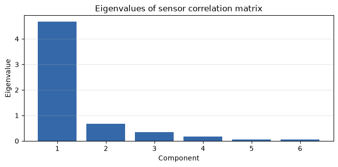
The eigenvector of the covariance matrix is a representative pattern where multiple sensors move simultaneously. Eigenvalues represent the magnitude of variation along that pattern. It can organize which combinations of equipment are dominant and use it to prioritize inspections.

Approach to Analysis and Modeling

For a square matrix $C$, a nonzero vector $v$ and a scalar $\lambda$

$Cv=\lambda v$

$\lambda$ is called eigenvalue, and $v$ is called eigenvector. Here, the standardized correlation matrix is used, making it less affected by differences at the sensor level. However, the sign of the eigenvector remains the same even if inverted.

Check with Python

Z = (sensor_df - sensor_df.mean()) / sensor_df.std(ddof=1)
C = Z.corr().to_numpy()
eigvals, eigvecs = np.linalg.eigh(C)
order = np.argsort(eigvals)[::-1]
eigvals, eigvecs = eigvals[order], eigvecs[:, order]
eig_table = pd.DataFrame({"eigenvalue": eigvals, "variance_ratio": eigvals / eigvals.sum()})
display(eig_table.round(4))

plt.figure(figsize=(7, 3.5))
plt.bar(np.arange(1, 7), eigvals, color="#3568a8")
plt.title("Eigenvalues of sensor correlation matrix")
plt.xlabel("Component")
plt.ylabel("Eigenvalue")
plt.grid(True, axis="y", alpha=0.3)
plt.tight_layout()
plt.show()

	eigenvalue	variance_ratio
0	4.6865	0.7811
1	0.6686	0.1114
2	0.3543	0.0590
3	0.1664	0.0277
4	0.0638	0.0106
5	0.0604	0.0101

Reading the results

If the first and second eigenvalues are larger than the others, it may be possible to explain the six sensor signals with a small number of common fluctuations. Before increasing individual alarms, it is effective to simultaneously inspect the sensor groups with high load on higher-level eigenvectors. Since the cause of failure cannot be determined based solely on eigenvalues, cross-reconciling with rotational speed, load, and maintenance history is necessary.

No.042: Exponentiation

Meaning in Practice

If you only want the maximum eigenvalues and corresponding vectors, the total eigenvalue calculation is excessive. The power method estimates the dominant vibration mode using only the repetition of the matrix and vector multiplication.

Approach to Analysis and Modeling

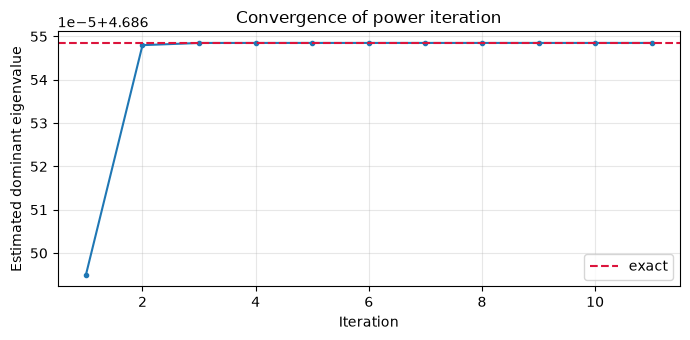
When iterating on $x_{k+1}=Cx_k/\|Cx_k\|_2$, if the initial value is not orthogonal to the maximum eigenvector and the absolute value of the maximum eigenvalue is unique, it converges in that direction. Eigenvalues are estimated using Rayleigh quotient $\lambda_k=x_k^TCx_k/(x_k^Tx_k)$. The convergence velocity depends on $|\lambda_2/\lambda_1|$.

Check with Python

x = np.ones(C.shape[0]) / np.sqrt(C.shape[0])
history = []
for k in range(30):
    x_new = C @ x
    x_new /= np.linalg.norm(x_new)
    lam = float(x_new @ C @ x_new)
    history.append(lam)
    if np.linalg.norm(x_new - x) < 1e-10 or np.linalg.norm(x_new + x) < 1e-10:
        x = x_new
        break
    x = x_new

display(pd.DataFrame({"sensor": sensor_names, "power_loading": x}).round(4))
print(f"iterations={len(history)}, estimate={lam:.6f}, exact={eigvals[0]:.6f}")
plt.figure(figsize=(7, 3.5))
plt.plot(range(1, len(history)+1), history, marker="o", ms=3)
plt.axhline(eigvals[0], color="crimson", linestyle="--", label="exact")
plt.title("Convergence of power iteration")
plt.xlabel("Iteration")
plt.ylabel("Estimated dominant eigenvalue")
plt.grid(True, alpha=0.3)
plt.legend()
plt.tight_layout()
plt.show()

	sensor	power_loading
0	Drive-X	0.4026
1	Drive-Y	0.3938
2	Bearing-A	0.4377
3	Bearing-B	0.4253
4	Frame	0.4090
5	Outlet	0.3782

iterations=11, estimate=4.686548, exact=4.686548

Reading the results

If the estimated value quickly approaches the exact calculation value, it is suitable for daily monitoring to update only the maximum mode. Since convergence is slower on equipment with close upper two eigenvalues, the upper limit of iterations and residual $\|Cx-\lambda x\|$ are monitored, and the ranchos method is switched to if necessary.

No.043: Reverse Repetition Method

Meaning in Practice

In resonance testing, the mode close to the design frequency, which is considered important, is not the maximum mode. The inverse iteration method selectively extracts eigenvalues near the specified value (shift).

Approach to Analysis and Modeling

Solve $(C-\mu I)y_k=x_k$ for shift $\mu$ and let $x_{k+1}=y_k/\|y_k\|$. In $(C-\mu I)^{-1}$, the component with the eigenvalue closest to $\mu$ dominates. If the shift is an eigenvalue itself, the matrix becomes singular, so check the numerical conditions.

Check with Python

shift = 0.50
x_inv = np.ones(C.shape[0]) / np.sqrt(C.shape[0])
inv_history = []
for k in range(20):
    y = np.linalg.solve(C - shift * np.eye(C.shape[0]), x_inv)
    x_inv = y / np.linalg.norm(y)
    lam_inv = float(x_inv @ C @ x_inv)
    residual = np.linalg.norm(C @ x_inv - lam_inv * x_inv)
    inv_history.append((k + 1, lam_inv, residual))
    if residual < 1e-10: break
display(pd.DataFrame(inv_history, columns=["iteration", "eigenvalue", "residual"]).tail().round(8))
print("nearest exact eigenvalue:", eigvals[np.argmin(np.abs(eigvals - shift))].round(6))

	iteration	eigenvalue	residual
15	16	0.3547	0.0110
16	17	0.3546	0.0095
17	18	0.3545	0.0082
18	19	0.3545	0.0071
19	20	0.3544	0.0062

nearest exact eigenvalue: 0.354291

Reading the results

Since it converges to the eigenvalue closest to the shift, it is suitable for mode exploration with a defined target bandwidth. In practice, it is not only confirmed that there is an eigenvalue in the targeted frequency but also that the sensor positions of the corresponding vectors overlap with the vibration frequencies derived from the rotational speed.

No.044: QR Method

Meaning in Practice

When you want to capture all eigenvalues with small to medium-scale models, the QR method is a fundamental technique. All modes of equipment models are displayed side by side to check proximity to hazardous bands.

Approach to Analysis and Modeling

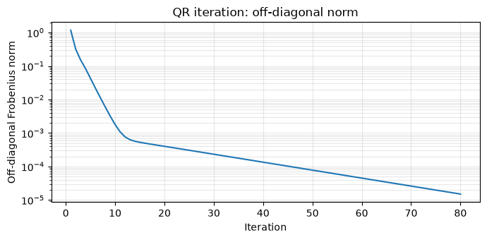
$A_k=Q_kR_k$ and QR decomposed, and updated with $A_{k+1}=R_kQ_k=Q_k^TA_kQ_k$. Since it is a similarity transformation, eigenvalues are preserved, and in symmetric matrices, diagonal components converge to eigenvalues through iteration. Practical libraries are being accelerated through shifts and Hessenberg transformations.

Check with Python

A_qr = C.copy()
offdiag_history = []
for k in range(80):
    Q, R = np.linalg.qr(A_qr)
    A_qr = R @ Q
    offdiag_history.append(np.linalg.norm(A_qr - np.diag(np.diag(A_qr))))
qr_vals = np.sort(np.diag(A_qr))[::-1]
display(pd.DataFrame({"QR_iteration": qr_vals, "numpy_eigh": eigvals, "abs_error": np.abs(qr_vals-eigvals)}).round(8))
plt.figure(figsize=(7, 3.5))
plt.semilogy(range(1, 81), offdiag_history)
plt.title("QR iteration: off-diagonal norm")
plt.xlabel("Iteration")
plt.ylabel("Off-diagonal Frobenius norm")
plt.grid(True, which="both", alpha=0.3)
plt.tight_layout()
plt.show()

	QR_iteration	numpy_eigh	abs_error
0	4.6865	4.6865	0.0000e+00
1	0.6686	0.6686	0.0000e+00
2	0.3543	0.3543	0.0000e+00
3	0.1664	0.1664	0.0000e+00
4	0.0638	0.0638	3.0000e-08
5	0.0604	0.0604	3.0000e-08

Reading the results

You can confirm that the norm of the non-diagonal component decreases and the diagonal value matches the eigenvalue of the ready-made function. The simple QR code method as teaching material is for checking the mechanism. In production, instead of repeating your own creations, you use well-verified numpy.linalg.eigh and similar materials.

No.045: The Ranchos Act

Meaning in Practice

Even if the covariance matrix of finite element models or many sensors is large, sometimes only the lower-order numerical modes are needed. The Lanchos method projects a symmetric matrix onto a small triple diagonal matrix.

Approach to Analysis and Modeling

Create a basis on the Krylov subspace $\mathcal{K}_m(A,q)=\mathrm{span}(q,Aq,\ldots,A^{m-1}q)$ and approximate the original eigenvalues with the eigenvalues (Ritz values) of $T_m=Q_m^TAQ_m$. Since finite-precision loses orthogonality, reorthogonalization is important in implementation.

Check with Python

n = 240
main = 2.2 + 0.15 * rng.random(n)
off = -1.0 * np.ones(n-1)
K = sparse.diags([off, main, off], [-1, 0, 1], format="csr")

def lanczos(A, m, seed=42):
    local_rng = np.random.default_rng(seed)
    q = local_rng.normal(size=A.shape[0]); q /= np.linalg.norm(q)
    Q, alphas, betas = [], [], []
    q_prev = np.zeros_like(q); beta = 0.0
    for j in range(m):
        Q.append(q.copy())
        z = A @ q - beta * q_prev
        alpha = float(q @ z); z -= alpha * q
        # To maintain numerical orthogonality in teaching materials, reorthogonality is performed on existing basis
        for qi in Q: z -= (qi @ z) * qi
        alphas.append(alpha)
        beta_new = np.linalg.norm(z)
        if beta_new < 1e-12: break
        if j < m-1: betas.append(beta_new)
        q_prev, q, beta = q, z / beta_new, beta_new
    return np.array(alphas), np.array(betas)

rows = []
exact_large = spla.eigsh(K, k=1, which="LA", return_eigenvectors=False)[0]
for m in [5, 10, 20, 30]:
    alpha, beta = lanczos(K, m)
    T = np.diag(alpha) + np.diag(beta, 1) + np.diag(beta, -1)
    ritz = np.linalg.eigvalsh(T)[-1]
    rows.append((m, ritz, abs(ritz-exact_large)))
display(pd.DataFrame(rows, columns=["Krylov_dim", "largest_Ritz", "abs_error"]).round(8))

	Krylov_dim	largest_Ritz	abs_error
0	5	4.1556	0.1362
1	10	4.2555	0.0363
2	20	4.2772	0.0145
3	30	4.2846	0.0071

Reading the results

Even with a 240-dimensional matrix, the maximum eigenvalues can be approximated from the much smaller Krylov subspace. In the equipment model, the acceptance criteria are the number of required modes, residuals, and calculation time. For models where symmetry is disrupted, the Arnoldy method is chosen instead of applying it as is.

No.046: Arnoldy Method

Meaning in Practice

The flow between processes is upstream and downstream, and the queues are generally asymmetrical. The Arnoldy method can approximate the main eigenvalues of models where reprocessing or delay propagates in a directional way.

Approach to Analysis and Modeling

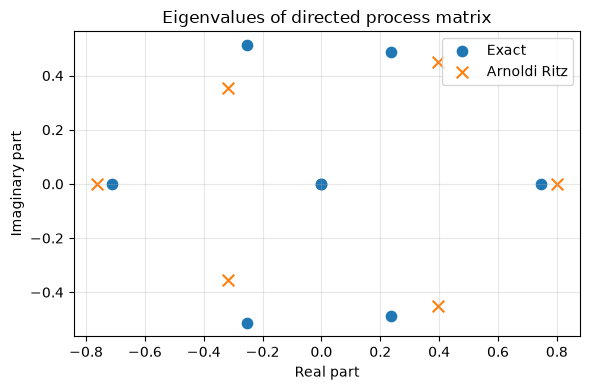
Arnoldi’s method constructs an orthonormal basis $Q_m$ of a Krylov subspace and projects onto the upper Hessenberg matrix $H_m$ that is $AQ_m\approx Q_mH_m$. It is positioned as an extension of the Lanchos method to asymmetric matrices. When complex eigenvalues appear, both absolute values and arguments are interpreted.

Check with Python

def arnoldi(A, m):
    n = A.shape[0]
    Q = np.zeros((n, m+1)); H = np.zeros((m+1, m))
    Q[:, 0] = np.ones(n) / np.sqrt(n)
    for k in range(m):
        v = A @ Q[:, k]
        for j in range(k+1):
            H[j, k] = Q[:, j] @ v
            v -= H[j, k] * Q[:, j]
        H[k+1, k] = np.linalg.norm(v)
        if H[k+1, k] < 1e-12: return H[:k+1, :k+1]
        Q[:, k+1] = v / H[k+1, k]
    return H[:m, :m]

H = arnoldi(A.T, 6)
ritz = np.linalg.eigvals(H)
exact = np.linalg.eigvals(A.T)
arnoldi_table = pd.DataFrame({
    "method": ["Arnoldi Ritz", "Exact"],
    "largest_abs_eigenvalue": [np.max(np.abs(ritz)), np.max(np.abs(exact))]
})
display(arnoldi_table.round(6))

plt.figure(figsize=(6, 4))
plt.scatter(exact.real, exact.imag, label="Exact", s=55)
plt.scatter(ritz.real, ritz.imag, marker="x", s=70, label="Arnoldi Ritz")
plt.title("Eigenvalues of directed process matrix")
plt.xlabel("Real part")
plt.ylabel("Imaginary part")
plt.grid(True, alpha=0.3)
plt.legend()
plt.tight_layout()
plt.show()

	method	largest_abs_eigenvalue
0	Arnoldi Ritz	0.8004
1	Exact	0.7457

Reading the results

You can see how the Ritz value of a small Hessenberg matrix captures the eigenvalues outside the original matrix. If there is an eigenvalue close to absolute value 1 in the process model, the influence may circulate and be less likely to attenuate. However, since the meaning changes depending on the matrix normalization rules, the weight is clearly indicated as probability or quantity.

No.047: Singular Value Decomposition

Meaning in Practice

Sensor data is a rectangular matrix. Singular Value Decomposition (SVD) divides into representative patterns in the temporal and sensor directions, and can be used to reduce storage capacity, remove noise, and extract representative waveforms.

Approach to Analysis and Modeling

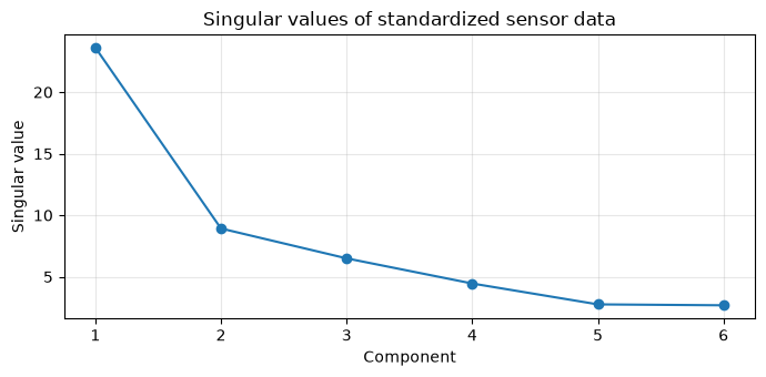
$Z=U\Sigma V^T$ Break it down. The singular value $\sigma_i$ is non-negative, and there is a $\sigma_i^2=\lambda_i$ between it and the eigenvalue of $Z^TZ$. $Z_k=U_k\Sigma_kV_k^T$ by the upper $k$ components is the best order $k$ approximation in the sense of the Frobenius norm.

Check with Python

U, s, Vt = np.linalg.svd(Z.to_numpy(), full_matrices=False)
svd_rows = []
for k in range(1, 7):
    Zk = U[:, :k] @ np.diag(s[:k]) @ Vt[:k, :]
    rel_error = np.linalg.norm(Z.to_numpy()-Zk, "fro") / np.linalg.norm(Z.to_numpy(), "fro")
    svd_rows.append((k, 1-rel_error, rel_error))
display(pd.DataFrame(svd_rows, columns=["rank", "reconstruction_score", "relative_error"]).round(4))

plt.figure(figsize=(7, 3.5))
plt.plot(range(1, 7), s, marker="o")
plt.title("Singular values of standardized sensor data")
plt.xlabel("Component")
plt.ylabel("Singular value")
plt.grid(True, alpha=0.3)
plt.tight_layout()
plt.show()

	rank	reconstruction_score	relative_error
0	1	0.5321	0.4679
1	2	0.6722	0.3278
2	3	0.7799	0.2201
3	4	0.8562	0.1438
4	5	0.8997	0.1003
5	6	1.0000	0.0000

Reading the results

If the singular values of the upper minority are large, the minority components can retain the main variation. Verify not only the compression ratio but also whether even the smallest signs just before failure have been eliminated. Reconstruction error can also be used as abnormal scores, but it is necessary to operate based solely on the normal period.

No.048: Relationship with PCA

Meaning in Practice

Principal Component Analysis (PCA) consolidates a large number of correlated monitoring values into a small number of uncorrelated KPIs. It can be used to reduce indicators on surveillance screens and to display equipment status in 2D.

Approach to Analysis and Modeling

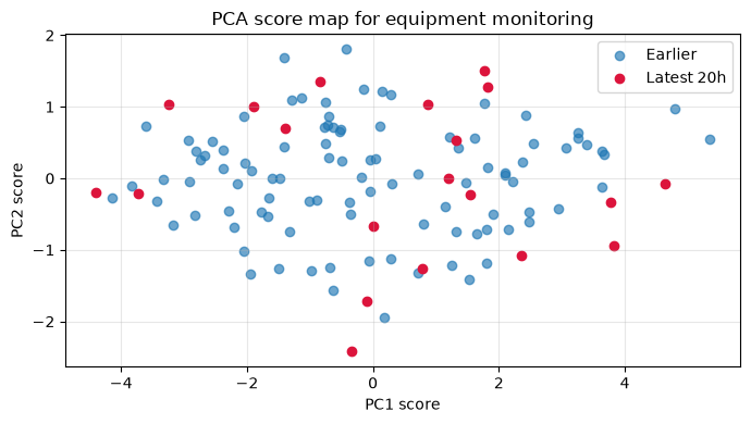
The method of eigenfactorizing the correlation matrix $C=Z^TZ/(n-1)$ of the normalized data $Z$ and SVD the $Z$ give the same principal component orientation. The contribution rate is $\lambda_j/\sum_i\lambda_i$. PCA is a method for explaining variance and is not necessarily the best predictor of quality defects.

Check with Python

scores = Z.to_numpy() @ eigvecs[:, :2]
loadings_df = pd.DataFrame(eigvecs[:, :2], index=sensor_names, columns=["PC1", "PC2"])
display(loadings_df.round(3))
print("Cumulative variance ratio (PC1+PC2):", round((eigvals[:2].sum()/eigvals.sum()), 4))

plt.figure(figsize=(7, 4))
plt.scatter(scores[:-20, 0], scores[:-20, 1], alpha=0.65, label="Earlier")
plt.scatter(scores[-20:, 0], scores[-20:, 1], color="crimson", label="Latest 20h")
plt.title("PCA score map for equipment monitoring")
plt.xlabel("PC1 score")
plt.ylabel("PC2 score")
plt.grid(True, alpha=0.3)
plt.legend()
plt.tight_layout()
plt.show()

	PC1	PC2
Drive-X	-0.403	0.558
Drive-Y	-0.394	0.600
Bearing-A	-0.438	-0.185
Bearing-B	-0.425	-0.302
Frame	-0.409	-0.336
Outlet	-0.378	-0.301

Cumulative variance ratio (PC1+PC2): 0.8925

Reading the results

The load scale indicates which sensor comprises each main component. If the point cloud from the last 20 hours is off from the past, it may be that the overall equipment condition has changed, not just a single sensor value. Management limits are not retrofitted to the same data; instead, the normal and verification periods are set separately.

No.049: Relationship with PageRank

Meaning in Practice

Measuring the importance of a process solely by the number of connections underestimates the processes affected by the critical process. PageRank performs a recursive evaluation, stating that the processes referenced and flowing into from the most important stages are also important.

Approach to Analysis and Modeling

Using the row probability matrix $P$, and the steady vector $r$

$r=\alpha P^Tr+(1-\alpha)v$

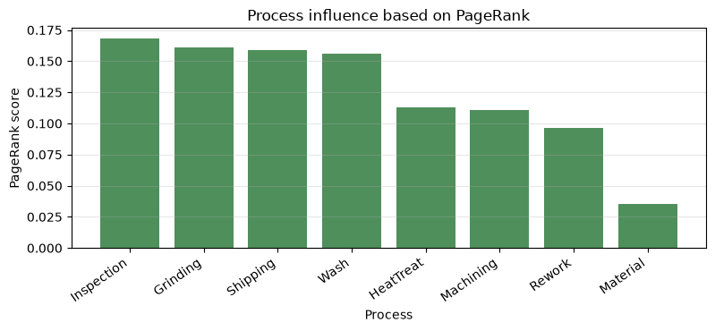
It is defined as follows. $\alpha$ is the probability of continuing network propagation, and $v$ is a uniform restart distribution. This is an eigenvector problem corresponding to the eigenvalue 1 of the Google matrix. Here, ranking is not process value, but structural importance on the defined link.

Check with Python

P = A.copy()
row_sum = P.sum(axis=1)
for i in range(len(P)):
    P[i] = P[i] / row_sum[i] if row_sum[i] > 0 else np.ones(len(P)) / len(P)
alpha = 0.85
G = alpha * P + (1-alpha) * np.ones_like(P) / len(P)
r = np.ones(len(P)) / len(P)
pr_history = []
for k in range(100):
    r_new = G.T @ r
    pr_history.append(np.linalg.norm(r_new-r, 1))
    if pr_history[-1] < 1e-12: break
    r = r_new
pagerank_df = pd.DataFrame({"process": processes, "PageRank": r_new}).sort_values("PageRank", ascending=False)
display(pagerank_df.round(4))

plt.figure(figsize=(8, 3.8))
plt.bar(pagerank_df["process"], pagerank_df["PageRank"], color="#4f8f5b")
plt.title("Process influence based on PageRank")
plt.xlabel("Process")
plt.ylabel("PageRank score")
plt.xticks(rotation=35, ha="right")
plt.grid(True, axis="y", alpha=0.3)
plt.tight_layout()
plt.show()

	process	PageRank
5	Inspection	0.1682
3	Grinding	0.1609
7	Shipping	0.1585
4	Wash	0.1560
2	HeatTreat	0.1130
1	Machining	0.1111
6	Rework	0.0967
0	Material	0.0356

Reading the results

If the process connecting to the reprocessing loop is a priority, it is a candidate to focus not only on direct losses at stoppage but also on ripple effects through circulation. Rankings depend on link weight and attenuation rate. Improvement investments multiply PageRank by throughput, downtime, substitability, and quality cost.

No.050: Applications to Graph Analysis

Meaning in Practice

By treating equipment and processes as nodes and relationships as edges, the entire factory can be treated as a graph. Spectral analysis identifies tightly linked processes, easily fragmented boundaries, and candidate monitoring units.

Approach to Analysis and Modeling

From the weight matrix $W$ that ignores direction, we create the degree matrix $D$ and Laplacian $L=D-W$. Normalized Laplacian

$L_{\mathrm{sym}}=I-D^{-1/2}WD^{-1/2}$

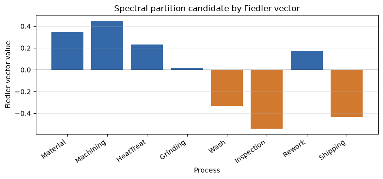
The smaller the second minimum eigenvalue (algebraic connectivity), the easier it is to split, and by the sign of the corresponding Fiedler vector, candidates for division into two groups can be obtained.

Check with Python

W = (A + A.T) / 2
d = W.sum(axis=1)
D_inv_sqrt = np.diag(1 / np.sqrt(d))
Lsym = np.eye(len(W)) - D_inv_sqrt @ W @ D_inv_sqrt
lap_vals, lap_vecs = np.linalg.eigh(Lsym)
fiedler = lap_vecs[:, 1]
cluster = np.where(fiedler >= 0, "Group A", "Group B")
graph_df = pd.DataFrame({"process": processes, "Fiedler_value": fiedler, "candidate_group": cluster})
display(graph_df.sort_values("Fiedler_value").round(4))
print("normalized algebraic connectivity:", round(lap_vals[1], 6))

plt.figure(figsize=(8, 3.8))
colors = np.where(fiedler >= 0, "#3568a8", "#d1792f")
plt.bar(processes, fiedler, color=colors)
plt.axhline(0, color="black", linewidth=0.8)
plt.title("Spectral partition candidate by Fiedler vector")
plt.xlabel("Process")
plt.ylabel("Fiedler vector value")
plt.xticks(rotation=35, ha="right")
plt.grid(True, axis="y", alpha=0.3)
plt.tight_layout()
plt.show()

	process	Fiedler_value	candidate_group
5	Inspection	-0.5414	Group B
7	Shipping	-0.4346	Group B
4	Wash	-0.3317	Group B
3	Grinding	0.0197	Group A
6	Rework	0.1728	Group A
2	HeatTreat	0.2314	Group A
0	Material	0.3464	Group A
1	Machining	0.4519	Group A

normalized algebraic connectivity: 0.183177

Reading the results

The two groups divided by code are candidates for consideration of maintenance responsibility scope, data collection units, and inter-process buffers. Edges connecting processes and groups near zero are candidate boundaries, but spectral splitting does not know physical layout or safety rules. Acceptance or rejection is decided by comparing with on-site traces.

Practical Implications Seen Through Target Exercise

1. You don’t have to calculate everything.: For maximum modes, you can narrow down the calculation to the proper eigenpairs needed for decision-making: exponential, symmetric large-scale, Ranchos method, and Asymmetric, Arnoldy’s method.
2. The same breakdown leads to multiple business operations.: Eigendecomposition and SVD serve as a common foundation for vibration modes, PCA, compression, and anomaly monitoring.
3. The definition of the network determines the conclusion: The ranking and division of PageRank and Laplacian vary depending on what is edged and what weight is applied.
4. Numerical results are not causes but candidates: Large eigenvalues or centrality indicate the priorities of the investigation but do not independently prove the cause of failures or quality defects.

What is necessary for practical implementation

• Data quality standards including sensor calibration, missing measurements, time synchronization, and equipment shutdown sections
• Verification data separating normal periods, abnormal periods, and load conditions
• Definition, standardization, shift, convergence tolerance, and recording random number seeds
• Acceptance criteria including residuals, reconstruction errors, calculation time, and false positive rates
• Review procedures for process managers, maintenance, and quality assurance to confirm results
• Workflow from alarm to inspection, cause confirmation, and model update

Conclusion

From No.041 to No.050, we examined the basics of eigenvalue problems, including exponential, inverse, QR methods, Krylov subspace methods, SVD/PCA, and PageRank/Graphaplasian through consistent hypothetical examples in manufacturing. What matters is not the advanced methodology name but the stable calculation of only the necessary information and translation into on-site inspection, investment, and monitoring design.

Consultations for Corporations

At Suri Kobo, we support everything from problem definition to implementation and operational design, covering equipment data analysis, anomaly detection, process network analysis, accelerated numerical calculations, and training for on-site personnel. We can work together with you on the verifying design to determine what can be made from on-hand data.

📩 Contact Us: surikobo.co.jp/contact
Please feel free to consult us first.