Capturing Temperature Changes and Energy in Continuous Furnaces Numerically: Numerical Integration and Differentiation Effective for Manufacturing Decision-Making with 10 Exercises (No.061–No.070)

In this article, we connect numerical derivatives, numerical integrals, automatic differentiation, and backpropagation methods to Early detection of temperature anomalies, grasping energy intensity, and sensitivity analysis of quality prediction models in a fictional heat treatment plant. Not only apply formulas, but also check how the notch width and measurement noise can alter your judgment.

[!NOTE] This material is a notebook previously used by Surikoubo (or personally by the representative, Kazuyama), and has been reconstructed, edited, and published with the company’s permission.
All data listed is fictional and has no relation whatsoever to real companies, factories, or figures.

Introduction: Practical Challenges in Manufacturing Covered in This Article

In continuous reactors, not only the current temperature but also “how quickly it has changed” and the instantaneous power value “how much is consumed over a certain period” are important. Furthermore, to improve quality forecasting models, it is necessary to calculate which operating conditions will significantly affect the predicted values. In this article, we will stably estimate the rate of change and cumulative amount from discrete measurements and translate them into operational decisions.

Common situations on site

• Only the temperature limit is monitored, missing sudden rises and drops
• The five-minute readings from the electricity meter are simply summed up, and the time units are mistaken.
• They always believe that using high-precision integration methods is beneficial, and do not check for data roughness or noise
• Quality prediction models work, but they cannot explain sensitivity or how they learn

Why is this issue so difficult to judge?

Field data are not continuous functions, but samples rounded at regular intervals and contain noise. Differentiation amplifies noise, while integration accumulates bias. Small notch widths are not always high precision; a balance between discretization and rounding errors is necessary. Also, the gradient obtained by automatic differentiation is a local sensitivity and cannot be interpreted as a causal effect as is.

Overview of Exercise covered this time

No.	Theme	Judgment in the manufacturing industry
061	Forward difference	Monitor the temperature rise rate online
062	central difference	Improving Change Rate with Historical Analysis
063	trapezoid formula	Calculating power consumption from measured power
064	Simpson’s rule	Achieving high precision in cumulative smooth load curves
065	Gaussian product	Heat load is evaluated using a small evaluation point
066	Romberg Points	Step-by-step accuracy verification and integration
067	error in numerical differentiation	Design of notch width and noise acceptance standards
068	automatic differentiation	Accurately calculating local sensitivity of quality models
069	backpropagation method	Confirm the learning principles of the quality prediction model
070	Implementation of Gradient Calculation	Quality assurance of model implementation through gradient verification

Preparing the Python environment

Numerical calculations are performed with NumPy and SciPy, tables with pandas, visualization with matplotlib, and automatic differentiation for PyTorch is used for No.068 to No.070. Fix the random number seed so you can reproduce the same result.

%matplotlib inline
import numpy as np
import pandas as pd
import matplotlib.pyplot as plt
import japanize_matplotlib
from scipy import integrate
from numpy.polynomial.legendre import leggauss
import torch

SEED = 20260712
rng = np.random.default_rng(SEED)
torch.manual_seed(SEED)
pd.set_option("display.precision", 4)
print(f"NumPy {np.__version__} / pandas {pd.__version__} / PyTorch {torch.__version__}")

NumPy 2.5.1 / pandas 3.0.3 / PyTorch 2.13.0

Creation of Fictional Data

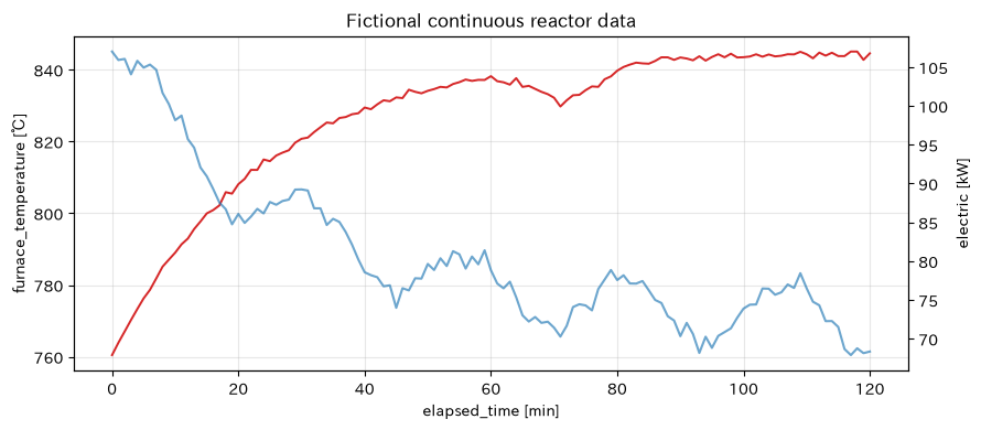
It simulates the 120-minute operation of a continuous furnace at one-minute intervals. The furnace temperature stabilizes after heating, and small disturbances occur around the 70-minute mark. Heater power includes temperature deviations and periodic load fluctuations. For explanation, both true values without noise and observed values with sensor noise added are retained.

t_min = np.arange(0, 121, dtype=float)
temp_true = 760 + 85 * (1 - np.exp(-t_min / 24)) - 9 * np.exp(-((t_min - 72) / 7) ** 2)
temp_obs = temp_true + rng.normal(0, 0.65, len(t_min))
power_kw = 72 + 35 * np.exp(-t_min / 30) + 4 * np.sin(2 * np.pi * t_min / 25) + rng.normal(0, 0.8, len(t_min))
furnace_df = pd.DataFrame({"elapsed_time_min": t_min, "furnace_temperature_true_value_c": temp_true,
                           "furnace_temperature_observation_c": temp_obs, "electric_kw": power_kw})
display(furnace_df.head())

fig, ax1 = plt.subplots(figsize=(9, 4))
ax1.plot(t_min, temp_obs, color="tab:red", lw=1.4, label="Furnace Temperature (Observation)")
ax1.set(title="Fictional continuous reactor data", xlabel="elapsed_time [min]", ylabel="furnace_temperature [℃]")
ax1.grid(alpha=0.3)
ax2 = ax1.twinx()
ax2.plot(t_min, power_kw, color="tab:blue", alpha=0.65, label="electric")
ax2.set_ylabel("electric [kW]")
fig.tight_layout()
plt.show()

	elapsed_time_min	furnace_temperature_true_value_C	furnace_temperature_observation_C	electric_kW
0	0.0	760.0000	760.4801	107.0138
1	1.0	763.4689	763.9120	105.9277
2	2.0	766.7962	767.0677	106.0636
3	3.0	769.9878	770.2546	104.0749
4	4.0	773.0491	773.3184	105.8155

No.061: Forward Differential

Meaning in Practice

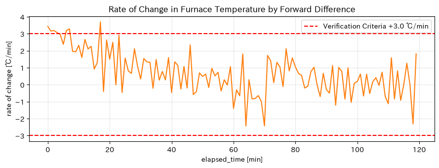
The forward difference is calculated by determining the rate of temperature change from the difference at adjacent points. It serves as the prototype for online monitoring that is easy to implement and updates every new measurement received.

Approach to Analysis and Modeling

Set the derivative of time $t$ with a step width $h$

$f'(t)\approx\frac{f(t+h)-f(t)}{h}$

It is similar to this. The discontinuation margin from Taylor’s deployment is $O(h)$. However, in actual operation, since the formula uses future values, when the value arrives, it is confirmed as the slope of the previous segment.

Check with Python

h = 1.0
forward_rate = np.diff(temp_obs) / h
rate_df = pd.DataFrame({"section_start_min": t_min[:-1], "forward_difference_c_per_min": forward_rate})
display(rate_df.loc[rate_df["forward_difference_c_per_min"].abs().nlargest(5).index].sort_values("section_start_min"))

plt.figure(figsize=(9, 3.5))
plt.plot(t_min[:-1], forward_rate, color="tab:orange")
plt.axhline(3.0, color="red", ls="--", label="Verification Criteria +3.0 ℃/min")
plt.axhline(-3.0, color="red", ls="--")
plt.title("Rate of Change in Furnace Temperature by Forward Difference")
plt.xlabel("elapsed_time [min]"); plt.ylabel("rate of change [℃/min]")
plt.grid(alpha=0.3); plt.legend(); plt.tight_layout(); plt.show()

	section_start_min	forward_difference_C_per_min
0	0.0	3.4319
2	2.0	3.1869
6	6.0	3.1885
7	7.0	3.2805
17	17.0	3.6901

Reading the results

At the initial stage of heating, the positive rate of change is large, and in the steady-state range, fine fluctuations caused by sensor noise become noticeable. A rate of change alarm can be a sign of an earlier temperature limit, but it does not stop at a single excess, and is combined with consecutive exceedances or moving averages. Thresholds are set for each product recipe and sensor accuracy.

No.062: Central Difference

Meaning in Practice

For post-event cause analysis, measurements from before and after can be used. The center difference is more accurate than the forward difference of the same increment width, making it suitable for detailed investigation of disturbance occurrence times and maximum heating speeds.

Approach to Analysis and Modeling

$f'(t)\approx\frac{f(t+h)-f(t-h)}{2h}$

The cancellation margin is $O(h^2)$. Since preceding and rearing noise are also subtracted, even if the true value is smooth and accurate, separate measures against observation noise are required. You cannot apply the formula at the endpoints.

Check with Python

central_obs = (temp_obs[2:] - temp_obs[:-2]) / (2 * h)
central_true = (temp_true[2:] - temp_true[:-2]) / (2 * h)
true_derivative = (85 / 24) * np.exp(-t_min / 24) + 18 * (t_min - 72) / 49 * np.exp(-((t_min - 72) / 7) ** 2)
comparison = pd.DataFrame({
    "technique": ["Forward difference (true value)", "Central difference (true value)"],
    "RMSE_C_per_min": [np.sqrt(np.mean((np.diff(temp_true) - true_derivative[:-1])**2)),
                         np.sqrt(np.mean((central_true - true_derivative[1:-1])**2))]
})
display(comparison)

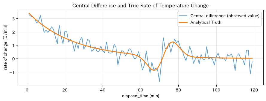
plt.figure(figsize=(9, 3.5))
plt.plot(t_min[1:-1], central_obs, label="Central difference (observed value)", alpha=0.7)
plt.plot(t_min[1:-1], true_derivative[1:-1], label="Analytical Truth", lw=2)
plt.title("Central Difference and True Rate of Temperature Change")
plt.xlabel("elapsed_time [min]"); plt.ylabel("rate of change [℃/min]")
plt.grid(alpha=0.3); plt.legend(); plt.tight_layout(); plt.show()

	technique	RMSE_C_per_min
0	Forward difference (true value)	0.0490
1	Central difference (true value)	0.0046

Reading the results

In noise-free data, the RMSE of the center difference is small, and accuracy improves as per theory. On the other hand, the curve of the observed values still shows fluctuations. If you prioritize real-time performance, you need to use one-sided differences; if you prioritize post-event accuracy, you need to use center differences.

No.063: Trapezoid Formula

Meaning in Practice

The process of calculating power consumption from instantaneous values in the electricity meter is numerical integration. The trapezoidal formula is a reliable method for connecting adjacent points with straight lines to calculate energy intensity by equipment and lot.

Approach to Analysis and Modeling

If we divide interval $[a,b]$ into $n$ and let $h=(b-a)/n$,

$\int_a^b f(t)dt\approx h\left(\frac{f_0}{2}+\sum_{i=1}^{n-1}f_i+\frac{f_n}{2}\right)$

That’s right. To integrate power [kW] with time [h] to obtain the amount of electricity [kWh], unit conversion by dividing minutes by 60 is essential.

Check with Python

energy_trap_kwh = np.trapezoid(power_kw, x=t_min / 60)
simple_sum_kwh = power_kw.sum() / 60
display(pd.DataFrame({"Calculation method": ["trapezoid formula", "Simple sum of each point"],
                      "value_120_minutes_of_electricity_kwh": [energy_trap_kwh, simple_sum_kwh]}))

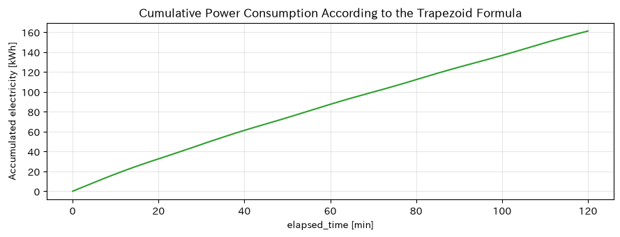
cumulative_kwh = integrate.cumulative_trapezoid(power_kw, t_min / 60, initial=0)
plt.figure(figsize=(9, 3.5))
plt.plot(t_min, cumulative_kwh, color="tab:green")
plt.title("Cumulative Power Consumption According to the Trapezoid Formula")
plt.xlabel("elapsed_time [min]"); plt.ylabel("Accumulated electricity [kWh]")
plt.grid(alpha=0.3); plt.tight_layout(); plt.show()

	Calculation method	120Electricity amount_kWh
0	trapezoid formula	161.1355
1	Simple sum of each point	162.5969

Reading the results

Simple sum counts points at both ends one by one, which differs from the trapezoidal formula. If the measurement interval is missing, the actual timestamp is passed to the integrator, not the number of lines. In unit intensity, this power is divided by the weight of good products and the number of units processed, and the range including setup and standby time is also standardized.

No.064: Simpson’s Law

Meaning in Practice

When the load curve is smooth and measured at equal intervals, Simpson’s law can accurately evaluate cumulative heat even with fewer measurement points. This is useful when comparing small differences in energy-saving measures.

Approach to Analysis and Modeling

Every two intervals, approximate the quadratic polynomial and denote the composite Simpson rule

$\int_a^b f(t)dt\approx\frac{h}{3}\left[f_0+f_n+4\sum_{i\in\mathrm{odd}}f_i+2\sum_{i\in\mathrm{even}}f_i\right]$

Let’s say so. The number of sections is even, with even intervals assumed. If smooth enough, the error is $O(h^4)$.

Check with Python

def smooth_power(t):
    return 72 + 35 * np.exp(-t / 30) + 4 * np.sin(2 * np.pi * t / 25)

reference, _ = integrate.quad(lambda x: smooth_power(x) / 60, 0, 120, epsabs=1e-12)
rows = []
for step in [20, 10, 5, 2]:
    grid = np.arange(0, 120 + step, step, dtype=float)
    y = smooth_power(grid)
    rows.append([step, np.trapezoid(y, grid / 60), integrate.simpson(y, x=grid / 60)])
accuracy_df = pd.DataFrame(rows, columns=["measurement_interval_min", "trapezoidal_kwh", "simpson_kwh"])
accuracy_df["trapezoid_absolute_error"] = abs(accuracy_df["trapezoidal_kwh"] - reference)
accuracy_df["simpson_absolute_error"] = abs(accuracy_df["simpson_kwh"] - reference)
display(accuracy_df)

	measurement_interval_min	trapezoid_kWh	simpson_kWh	trapezoid_absolute_error	simpson_absolute_error
0	20	161.1771	160.4518	0.1857	9.1099e-01
1	10	161.4131	161.4918	0.0503	1.2900e-01
2	5	161.3777	161.3659	0.0150	3.1844e-03
3	2	161.3653	161.3628	0.0025	6.8897e-05

Reading the results

With this smooth simulated curve, the error of Simpson’s Law is smaller at the same measurement interval. However, if measured noise or missing measurements dominate, the theoretical accuracy of higher-order formulas does not directly translate into operational accuracy. Compare instrument accuracy and the impact of data interpolation as well.

No.065: Gaussian Multiplication

Meaning in Practice

In cases like heat conduction simulations, where a single function evaluation is expensive, there are situations where it is better to select points with a larger amount of information than to evaluate many at equal intervals. Gaussian multiplication aims for high accuracy with only a few evaluation points.

Approach to Analysis and Modeling

$n$ The Gauss–Legendre product of point Gauss–Legendre uses the root $x_i$ and weight $w_i$ of the Legendre polynomial on interval $[-1,1]$,

$\int_{-1}^{1}f(x)dx\approx\sum_{i=1}^n w_i f(x_i)$

Let’s say so. $2n-1$ Polynomials of the following order are strict. Variable conversion is performed for general intervals.

Check with Python

def gauss_integral(func, a, b, n):
    x, w = leggauss(n)
    mapped = (b - a) * x / 2 + (a + b) / 2
    return (b - a) / 2 * np.sum(w * func(mapped))

gauss_rows = []
for n in [2, 3, 4, 6, 8]:
    estimate = gauss_integral(lambda x: smooth_power(x) / 60, 0, 120, n)
    gauss_rows.append([n, estimate, abs(estimate - reference)])
display(pd.DataFrame(gauss_rows, columns=["Evaluation Score", "power_consumption_kwh", "absolute_error_kwh"]))

	Evaluation Score	power_consumption_kWh	absolute_error_kWh
0	2	156.9831	4.3797
1	3	164.9006	3.5378
2	4	163.9079	2.5451
3	6	157.8160	3.5467
4	8	160.2179	1.1449

Reading the results

Increasing the evaluation score brings you closer to the reference value. Since the evaluation points for Gaussian integration do not match the actual periodic sensor time, they are more suitable for simulations and design calculations where evaluation times can be selected, rather than aggregating existing logs. If there are discontinuities or steep changes, segments are divided.

No.066: Romberg Points

Meaning in Practice

If you want to check not only the value of numerical integration but also the convergence when the increments are fine, the Romberg integral is helpful. It can explain the accuracy of heat balance calculations step by step, helping to build consensus on calculation time and accuracy.

Approach to Analysis and Modeling

Create a trapezoidal formula $R_{k,0}$ with the increment width halved, and use Richardson interpolation

$R_{k,j}=R_{k,j-1}+\frac{R_{k,j-1}-R_{k-1,j-1}}{4^j-1}$

to cancel out the main error terms. It is a smooth function with high convergence, but it is not intended to arbitrarily supplement measurement sequences containing noise.

Check with Python

def romberg_table(func, a, b, levels=6):
    R = np.zeros((levels, levels))
    for k in range(levels):
        n = 2**k
        x = np.linspace(a, b, n + 1)
        R[k, 0] = np.trapezoid(func(x), x)
        for j in range(1, k + 1):
            R[k, j] = R[k, j-1] + (R[k, j-1] - R[k-1, j-1]) / (4**j - 1)
    return R

R = romberg_table(lambda x: smooth_power(x) / 60, 0, 120, levels=7)
romberg_df = pd.DataFrame(R).mask(np.triu(np.ones_like(R, dtype=bool), 1))
romberg_df.index.name = "Levels of Subdivision k"
romberg_df.columns = [f"Extrapolating order j={j}" for j in range(R.shape[1])]
display(romberg_df.round(8))
print(f"Final estimate: {R[-1,-1]:.8f} kWh / Difference from reference value: {abs(R[-1,-1]-reference):.2e} kWh")

	Extrapolating order j=0	Extrapolating order j=1	Extrapolating order j=2	Extrapolating order j=3	Extrapolating order j=4	Extrapolating order j=5	Extrapolating order j=6
Levels of Subdivision k
0	175.8368	NaN	NaN	NaN	NaN	NaN	NaN
1	167.0063	164.0628	NaN	NaN	NaN	NaN	NaN
2	163.5388	162.3830	162.2711	NaN	NaN	NaN	NaN
3	161.4236	160.7186	160.6076	160.5812	NaN	NaN	NaN
4	161.3944	161.3846	161.4290	161.4420	161.4454	NaN	NaN
5	161.3714	161.3637	161.3623	161.3612	161.3609	161.3608	NaN
6	161.3650	161.3628	161.3628	161.3628	161.3628	161.3628	161.3628

Final estimate: 161.36277623 kWh / Difference from reference value: 1.10e-05 kWh

Reading the results

If the value stabilizes as you move toward the lower right of the table, you can judge that the discretization error is being controlled. In actual testing, the gap between adjacent levels falls below the operational tolerance limit. It’s not about increasing the number of digits itself, but about aligning with the accuracy of the electric meter and the range of energy-saving measures being determined.

No.067: Error in Numerical Differentiation

Meaning in Practice

In differentiation, finer chopping does not always guarantee better results. If the increments are large, discretization errors occur; if too small, floating-point drops and measurement noise dominate. This forms the basis for determining the monitoring cycle and smoothing range.

Approach to Analysis and Modeling

The cutoff error for the center difference is generally $C_1h^2$, and the rounding error is about $C_2\varepsilon/h$. The total error forms a U-shape, and there is an optimal notch width. In actual measurements, sensor noise can be much greater than the rounding error.

Check with Python

x0 = 1.0
hs = np.logspace(-16, -1, 80)
exact = np.cos(x0)
errors64 = np.array([abs((np.sin(x0+h)-np.sin(x0-h))/(2*h) - exact) for h in hs])
rng_noise = np.random.default_rng(SEED)
noise_level = 1e-5
errors_noisy = []
for h_ in hs:
    yp = np.sin(x0+h_) + rng_noise.normal(0, noise_level)
    ym = np.sin(x0-h_) + rng_noise.normal(0, noise_level)
    errors_noisy.append(abs((yp-ym)/(2*h_) - exact))

plt.figure(figsize=(8, 4))
plt.loglog(hs, errors64, label="floating-point only")
plt.loglog(hs, errors_noisy, label="Contains slight measurement noise", alpha=0.75)
plt.title("Notch Width and Error in Central Difference")
plt.xlabel("Notch width h"); plt.ylabel("absolute_error")
plt.grid(True, which="both", alpha=0.3); plt.legend(); plt.tight_layout(); plt.show()
print(f"Best Notch Width for Floating-Point Only: {hs[np.argmin(errors64)]:.2e}")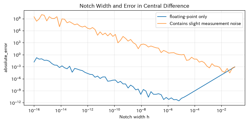

Best Floating-Point Notch Width: 6.65E-06

Reading the results

Even without noise, inflated increments that are too small can increase errors, and amplification becomes even more pronounced when noise is present. In equipment monitoring, before shortening the sampling cycle, sensor resolution, detection delays due to smoothing, and the time scale of changes to be detected are evaluated together.

No.068: Automatic Differentiation

Meaning in Practice

To understand how much defect risk changes when moving the furnace temperature by 1°C in quality prediction models, a gradient is necessary. Automatic differentiation does not specify the notch width of finite differences, but finds the derivative with mechanical accuracy along the calculated graph.

Approach to Analysis and Modeling

Let the prediction score be $s=0.018(T-820)^2+0.12v^2+0.004(T-820)v$. Automatic differentiation combines the local derivatives of each operation, such as addition and multiplication, using the chain law. This is neither a symbolic transformation of a formula nor a finite difference.

Check with Python

T = torch.tensor(828.0, requires_grad=True)
v = torch.tensor(1.8, requires_grad=True)
score = 0.018 * (T - 820)**2 + 0.12 * v**2 + 0.004 * (T - 820) * v
score.backward()
autograd_df = pd.DataFrame({"variable": ["furnace_temperature T [℃]", "transport speed v [m/min]"],
                            "present value": [T.item(), v.item()],
                            "local gradient": [T.grad.item(), v.grad.item()]})
display(autograd_df)

	variable	present value	local gradient
0	furnace_temperature T [℃]	828.0	0.2952
1	transport speed v [m/min]	1.8	0.4640

Reading the results

The sign for the local gradient indicates the direction of score change when the variable is increased around the current point. Absolute values of gradients with different units are not directly compared; instead, the realistic change is multiplied by the effect amount. Also, the gradient of the observation model is a local sensitivity based on correlation and does not guarantee causal effects of manipulation.

No.069: Backpropagation Method

Meaning in Practice

Backpropagation is at the core of training neural networks. The error between the quality prediction value and the actual result is distributed from the output side to each weight, and the direction in which direction the update should be calculated.

Approach to Analysis and Modeling

Let a model with a single hidden layer $\hat y=W_2\tanh(W_1x+b_1)+b_2$ and mean squared error be $L=n^{-1}\sum(\hat y-y)^2$. Inverse mode automatic differentiation efficiently propagates from $\partial L/\partial W_2$ to the preceding gradient by the chain law.

Check with Python

n = 120
X_np = np.column_stack([rng.normal(820, 8, n), rng.normal(1.8, 0.25, n)])
y_np = 0.018*(X_np[:,0]-820)**2 + 0.12*X_np[:,1]**2 + 0.004*(X_np[:,0]-820)*X_np[:,1]
y_np += rng.normal(0, 0.08, n)
X = torch.tensor((X_np - X_np.mean(0))/X_np.std(0), dtype=torch.float32)
y = torch.tensor(y_np[:, None], dtype=torch.float32)

model = torch.nn.Sequential(torch.nn.Linear(2, 6), torch.nn.Tanh(), torch.nn.Linear(6, 1))
optimizer = torch.optim.Adam(model.parameters(), lr=0.03)
losses = []
for epoch in range(301):
    optimizer.zero_grad()
    loss = torch.mean((model(X) - y)**2)
    loss.backward()
    optimizer.step()
    losses.append(loss.item())

plt.figure(figsize=(8, 3.5))
plt.plot(losses)
plt.title("Training Quality Prediction Models Using Backpropagation Methods")
plt.xlabel("epoch"); plt.ylabel("mean squared error")
plt.grid(alpha=0.3); plt.tight_layout(); plt.show()
print(f"initial loss: {losses[0]:.4f} / Final loss: {losses[-1]:.4f}")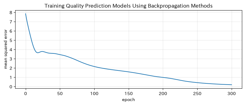

Initial loss: 7.8346 / Final loss: 0.1815

Reading the results

Losses decrease, and you can see that the gradient calculated by backpropagation is working well for learning. However, training losses alone are not enough to decide on hiring. We evaluate the losses caused by operating decisions caused by verification by equipment, product type, and period, overlearning monitoring, and prediction errors.

No.070: Implementation of Gradient Calculation

Meaning in Practice

Errors in gradient implementation can cause the model to fail to learn or to recommend incorrect operating conditions. Gradient checks that match self-made analytical gradients, automatic differentiation, and finite differences serve as acceptance tests for analysis codes.

Approach to Analysis and Modeling

Let the loss of linear regression be $L(w)=n^{-1}\|Xw-y\|_2^2$, then the analytical gradient is

$\nabla_wL=\frac{2}{n}X^T(Xw-y)$

That’s right. Approximate each component using central differences, compare the results of automatic differentiation with relative errors. Finite differences are for verification purposes, and the computational complexity is too large for large-scale learning bodies.

Check with Python

X_check = np.column_stack([np.ones(8), np.linspace(-1, 1, 8), np.linspace(-1, 1, 8)**2])
y_check = np.array([1.5, 1.2, 1.0, 0.9, 1.0, 1.3, 1.7, 2.2])
w = np.array([1.0, -0.2, 0.5])

def mse_np(w_):
    return np.mean((X_check @ w_ - y_check)**2)

analytic = 2 / len(y_check) * X_check.T @ (X_check @ w - y_check)
eps = 1e-6
finite = np.array([(mse_np(w + eps*np.eye(3)[j]) - mse_np(w - eps*np.eye(3)[j]))/(2*eps) for j in range(3)])
wt = torch.tensor(w, dtype=torch.float64, requires_grad=True)
Xt = torch.tensor(X_check, dtype=torch.float64)
yt = torch.tensor(y_check, dtype=torch.float64)
torch.mean((Xt @ wt - yt)**2).backward()
auto = wt.grad.detach().numpy()

gradient_df = pd.DataFrame({"coefficient": ["slice", "Linear term", "Quadratic term"], "analytical gradient": analytic,
                            "finite difference": finite, "automatic differentiation": auto,
                            "analysis_vs_automatic_absolute_difference": abs(analytic-auto)})
display(gradient_df)
print(f"Maximum difference in gradient check: {np.max(abs(analytic-auto)):.2e}")

	coefficient	analytical gradient	finite difference	automatic differentiation	Analysisvsautomatic_absolute_difference
0	slice	-0.2714	-0.2714	-0.2714	0.0
1	Linear term	-0.4714	-0.4714	-0.4714	0.0
2	Quadratic term	-0.2294	-0.2294	-0.2294	0.0

Maximum gradient check difference: 0.00e+00

Reading the results

If the three methods match with sufficiently small margins, the basic integrity of gradient implementations can be confirmed. In production, random multiple points, near boundaries, and non-smooth points in the activation function are also tested, and tolerances are determined according to the data type. Gradient check is not about model accuracy, but about assessing the validity of implementation.

Practical Implications Seen Through Target Exercise

1. Change rate and cumulative amount capture different anomalies: Differentiation visualizes sudden changes, while integration visualizes small deviations over long periods.
2. Prerequisites are more important than higher-order methods: If the spacing, smoothness, noise, and endpoint processing are compromised, theoretical accuracy cannot be achieved.
3. Accuracy is determined by the task unit: Convert numerical errors into power consumption, cost, temperature deviation, and quality loss, and determine the required magnitudes.
4. Gradient is the local sensitivity of the model: Before using them for operational recommendations, check constraints, interactions, causality, and data scope.

What is necessary for practical implementation

• Sensor calibration, time synchronization, missing measurements, unit, and sampling cycle management
• Operational context that distinguishes recipe changes, scheduling, and stoppage intervals
• Clarification of notch width, interpolation, smoothing, endpoint processing, and convergence tolerance
• Unit tests and regression tests using analytical values, automatic differentiation, and finite differences
• Acceptance criteria separating numerical error, measurement error, and model error
• Workflow for post-alarm confirmation, operational permissions, safety restrictions, and model updates

Conclusion

In No.061 to No.070, we confirmed the rate of change due to forward and central differences, cumulative quantities according to trapezoidal shapes, Simpson Gauss, and Romberg, automatic differentiation, backpropagation, and gradient checks using consistent hypothetical examples of continuous reactors. What matters is not just the official order of accuracy, but also choosing methods that match the nature of the data and the tolerance for error in decision-making, and operating them in a verifiable form.

Consultations for Corporations

At Mathematical Laboratory, we support everything from problem organization to implementation and operational design, covering everything from numerical analysis of manufacturing data, energy intensity design, equipment anomaly detection, quality prediction models, gradient-based optimization, to on-site staff training.

📩 Contact Us: surikobo.co.jp/contact
Please feel free to consult us first.