100 Python Exercises for Data Analysis

This is a series where you can systematically learn data analysis skills using Python using 100 Exercises, using on-site data from the manufacturing industry as the subject matter.
This series is designed by Surikobo for people in the manufacturing industry and those in charge of DX promotion.

[!NOTE] This material is a notebook that has been used in corporate training by Surikobo (or its representative, Hiroshi Wayama) in the past, and has been reorganized and edited with the permission of the company and published.
All published data is fictitious and has no relation to actual companies, factories, or numbers.

---

Purpose of the series

A huge amount of data is accumulated every day at manufacturing sites, including production numbers, defect rates, and equipment utilization rates.
However, the situation of “We have data, but we are not making use of it” is a common problem in many workplaces.

The purpose of this series is to develop the ability to solve on-site data analysis issues while learning Python from scratch.
Each exercise deals with a specific theme that is relevant to practical work, and aims to provide content that you can try out in the field from the day you finish reading it.

---

Composition of 10 chapters

Chapter	Title	Exercise	Main Topic
Chapter 1	Python preparation and basics	No.001~010	Execution environment, print, how to read errors, flow of analysis
Chapter 2	Variables, types, and operations	No.011-020	Numerical values, character strings, truth/false values, four arithmetic operations, and comparison operations
Chapter 3	Strings, lists, and dictionaries	No.021-030	Basics of string operations, lists, and dictionaries
Chapter 4	Conditional branching and repetition	No.031-040	if statements, for statements, while statements, and rank determination
Chapter 5	Functions, modules, and exception handling	No.041-050	Function definitions, standard libraries, try-except
Chapter 6	File operations and CSV	No.051-060	File reading/writing/CSV operations/Monthly aggregation
Chapter 7	Introduction to NumPy	No.061-070	Array operations, statistical calculations, and condition extraction
Chapter 8	Introduction to Polars	No.071~080	Series/DataFrame/CSV reading
Chapter 9	Data processing using Polars	No.081-090	Column operations, missing value processing, sorting, and duplicate removal
Chapter 10	Aggregation/Visualization/Mini analysis	No.091~100	group_by/Matplotlib/Correlation/Analysis report

---

Positioning of this notebook

This notebook corresponds to Chapter 1 (No.001-No.010).

• Theme: Automotive parts factory 3rd line 2024 Q1 production results (fictional data)
• Goal: What is Python, how to set up the execution environment, and experience the first steps of basic syntax
• Time required: Approximately 60 minutes
• Libraries used: NumPy, Matplotlib (no external data required)

---

Learn Python using production line operation data

100 Exercises Chapter 1 (No.001 to No.010): Python preparation and basics

Data on production volume, defect rate, and equipment utilization rate continues to accumulate at the manufacturing site.
“We have data, but we are not using it.” In order to solve such on-site issues, This is the first chapter of 100 Exercises on learning Python from scratch.

This article covers the following 10 exercises.

No.	Title
001	Understand what you can do with Python
002	Organizing the reasons why Python is used in data analysis
003	Preparing the Python execution environment
004	Understand the basic operations of Jupyter Notebook
005	Run a Python script
006	Displaying characters with the print function
007	Write a comment
008	Understanding how to read error displays
009	Executing code cells separately
010	Understand the basic flow of data analysis

Target audience: Manufacturing industry personnel and DX promotion personnel with no Python experience Time required: Approximately 60 minutes Libraries used: NumPy, Matplotlib (no external data required)

Introduction: Practical issues in the manufacturing industry covered in this article

Overview of target factories/issues

In this article, we will discuss the third line of a small and medium-sized manufacturing industry that manufactures automobile parts.

• Factory size: 200 employees, manufacturing of metal parts for automobiles
• Issue: Not being able to analyze daily production reports that are manually entered into Excel every day.
• Data: Daily production volume, number of defective products, equipment utilization rate (manual input Excel data)

Currently, at the end of each month, a person in charge compiles the data in Excel and creates a graph. By the time I noticed it, it was the end of the month.'' I can see a trend, but it doesn’t serve as a basis for countermeasures.”

Common situations in the field

Situation	Actual problem
Data is managed in Excel	There are so many sheets that it takes 1 to 2 hours to aggregate
Monthly reports are done manually	Prone to human error
It is too late to notice changes in the defect rate	Month-end tabulation does not allow countermeasures to be taken in time for the following month
Equipment maintenance is “repair after it breaks”	Large opportunity loss due to failure to perform preventive maintenance
Absence of person in charge of analysis	Issues accumulate without anyone learning Python

In all of these situations, you have the data, you’re motivated, but you can’t do anything about it.
You can change this by simply learning the basics of Python.

Why is this problem difficult to judge?

Dilemma of “tool selection” and “learning cost”

There is a wall that many field personnel run into when starting to use Python.

1. I don’t know which materials to study with The introductory book starts with “Hello World,” but there is no visible connection to the data on the manufacturing floor.

2. Stuck with environment construction Anaconda, pip, venv… There are so many terms that it’s easy to get frustrated before you even get started.

3. I can’t see if it can be used for my work There is a lot of abstract sample code, which makes me feel like it’s not relevant to me in the manufacturing industry.

4. It is difficult to experience small successes If you aim for a finished product (machine learning/dashboard) first, you will be disappointed.

In this exercise series, we give top priority to “quickly writing code that works with data from the manufacturing site”.

Overall picture of the exercises covered in this chapter

Position of Chapter 1

Chapter 1 (this time): Python preparation and basics ← here
Chapter 2: Variables, types, and operations
Chapter 3: Strings, Lists, and Dictionaries
Chapter 4: Conditional branching and repetition
Chapter 5: Functions, Modules, and Exception Handling
Chapter 6: File operations and CSV
Chapter 7: Introduction to NumPy
Chapter 8: Introduction to Polars
Chapter 9: Data processing with Polars
Chapter 10: Aggregation/Visualization/Mini-analysis

Learning roadmap for No.001~010

[No.001-002] Get an overview of Python
      ↓
[No.003-004] Prepare the environment and start using Jupyter
      ↓
[No.005-006] Write and run the first code
      ↓
[No.007-008] Get into the habit of writing code correctly
      ↓
[No.009-010] Divide the code and get the overall picture of the analysis

In No.010, you will apply what you have learned so far to experience actual data analysis flow on a manufacturing line.

Preparing the Python environment

Execution environment

This notebook has been confirmed to work in the following environments.

!sw_vers

ProductName:		macOS
ProductVersion:		26.3
BuildVersion:		25D125

!python -V

Python 3.13.1

Import the required libraries and check their versions.

%matplotlib inline
%config InlineBackend.figure_format = 'svg'

import random
import sys
import platform

import numpy as np
import matplotlib
import matplotlib.pyplot as plt

# Fixed random number seed (ensuring reproducibility)
seed = 42
random.seed(seed)
np.random.seed(seed)

# Japanese font settings
if platform.system() == 'Darwin':
    matplotlib.rcParams['font.family'] = 'Hiragino Maru Gothic Pro'
elif platform.system() == 'Linux':
    matplotlib.rcParams['font.family'] = 'IPAGothic'
matplotlib.rcParams['axes.unicode_minus'] = False

print(f"Python     : {sys.version.split()[0]}")
print(f"NumPy      : {np.__version__}")
print(f"Matplotlib : {matplotlib.__version__}")
print(f"OS         : {platform.system()} {platform.release()}")

Python     : 3.13.1
NumPy      : 2.5.1
Matplotlib : 3.11.0
OS         : Darwin 25.3.0

Creation of fictitious data

Data background

In this article, we will introduce the 2024 Q1 (January to March, 90 days) of Automotive parts factory 3rd line. Uses actual production data. All data is generated on the fly in Python (no external files required).

Variable name	Content	Unit
production	Daily production	Units
defects	Number of defective items by day	pcs
defect_rate_pct	Daily defect rate	%
operation_rate	Daily equipment utilization rate	%

This data will be used in No.009 and No.010. No.001 to 008 are code examples for each exercise alone.

# Fictional data: Auto parts factory 3rd line 2024 Q1 production results
np.random.seed(42)

n_days = 90  # 2024 Q1 (January to March)
day_index = np.arange(1, n_days + 1)

# Daily production number (target 1,000 units/day, random fluctuation of ±10%)
production = (1000 + np.random.normal(0, 80, n_days)).astype(int)
production = np.clip(production, 750, 1200)

# Defect rate (monthly cycle trend + Gaussian noise)
true_defect_rate = 0.020 + 0.008 * np.sin(day_index * 2 * np.pi / 30)
defects = np.round(production * true_defect_rate + np.random.normal(0, 2, n_days)).astype(int)
defects = np.clip(defects, 0, production // 10)
defect_rate_pct = defects / production * 100

# Equipment utilization rate (%)
operation_rate = 94 - 2 * np.cos(day_index * 2 * np.pi / 30) + np.random.normal(0, 1.5, n_days)
operation_rate = np.clip(operation_rate, 82, 99)

print("Overview of fictitious data")
print("=" * 45)
print(f"  period       : 2024yearQ1({n_days}days)")
print(f"  Total production number   : {production.sum():>8,} stand")
print(f"  Total number of defective items : {defects.sum():>8,} units")
print(f"  Average defect rate : {defect_rate_pct.mean():>8.2f} %")
print(f"  Average occupancy rate : {operation_rate.mean():>8.1f} %")

Overview of fictitious data ============================================= Period: Q1 2024 (90 days) Total production: 89,243 units Total number of defective items: 1,799 pieces Average defect rate: 2.01% Average occupancy rate: 94.0%

---

No.001: Understand what you can do with Python

Practical meaning

It is important to understand specifically how Python can help improve operations in the manufacturing industry. This is the most important motivation to continue learning.

Even if the word “programming” sounds difficult, The essence of what we do with Python is to automate repetitive tasks. “Reading trends from data” are two points.

Concept of analysis and modeling

Data utilization in the manufacturing industry will be easier to organize if you consider the following four steps.

1. Collect: Load sensor and manual input data with Python
2. Maintenance: Correct missing values, outliers, and format inconsistencies
3. Analysis: Grasp trends with aggregation, visualization, and statistical models
4. Utilization: KPI monitoring, prediction, optimization, and automated reporting

Python is a tool that automates and speeds up these four steps.

Check with Python

Categorize and list the problems that Python can solve in the manufacturing industry.

# No.001: Understand what you can do with Python

categories = {
    "Data collection and maintenance": [
        "Load and combine CSV/Excel files",
        "Real-time acquisition of sensor data",
        "Connection/query with database (SQL)",
    ],
    "Aggregation/statistical analysis": [
        "Daily/monthly tally of production numbers and defect rates",
        "Correlation analysis between processes",
        "Automatic creation of control charts (Xbar-R control charts)",
    ],
    "Prediction/machine learning": [
        "Detection of signs of defective products",
        "Predictive maintenance (PdM) of equipment",
        "Optimization of production planning through demand forecasting",
    ],
    "Automation/Reporting": [
        "Automatic generation and email of daily reports",
        "Building a web dashboard",
        "API integration with Manufacturing Execution System (MES)",
    ],
}

print("Categories of manufacturing problems that can be solved with Python")
print("=" * 55)
total = 0
for category, items in categories.items():
    print(f"\n▶ {category}")
    for item in items:
        print(f"   ・{item}")
        total += 1
print(f"\nTotal: {total} Usage example")

Categories of manufacturing problems that can be solved with Python ========================================================

▶ Data collection and maintenance
   ・Load and combine CSV/Excel files
   ・Real-time acquisition of sensor data
   ・Connection/query with database (SQL)

▶ Aggregation/statistical analysis
   ・Daily/monthly aggregation of production numbers and defect rates
   ・Correlation analysis between processes
   ・Automatic creation of control chart (Xbar-R control chart)

▶ Prediction/machine learning
   ・Detection of signs of defective products
   ・Predictive maintenance (PdM) of equipment
   ・Optimization of production planning through demand forecasting

▶ Automation/Reporting
   ・Automatic generation and email sending of daily reports
   ・Building a web dashboard
   ・API cooperation with manufacturing execution system (MES)

Total: 12 usage examples

Reading the results

Looking at the output, the areas where Python is used range from “data collection” to “automation”. You can see that it is covered cross-sectionally.

Particularly in the manufacturing industry, the field of aggregation and statistical analysis is highly effective.
The experience of being able to finish monthly aggregation in 5 seconds, which used to take 2 hours, This will be your biggest motivation to continue learning Python.

From the perspective of DX promotion: First, we will summarize the existing Excel data using Python. Set small goals and move toward prediction and automation while accumulating successful experiences. A step-up approach is effective.

---

No.002: Organize the reasons why Python is used in data analysis

Practical meaning

If you can’t explain why you use Python instead of Excel, It will be difficult to introduce tools without involving superiors and colleagues.
Organizing comparisons with other tools will serve as the basis for a proposal to introduce Python within your company.

Concept of analysis and modeling

When comparing data tools commonly used in the manufacturing industry, their positions are as follows.

• Excel: Excellent for aggregating, creating graphs, and sharing small amounts of data. I don’t like large amounts of data or automation.
• SQL: Powerful for database aggregation and extraction. I often call SQL from Python.
• R: Specialized in statistical analysis. Although it is on par with Python, Python has a rich set of engineering libraries.
• Python: A general-purpose language that covers everything from data analysis to system development. Learning costs are low.

Check with Python

Displays the characteristics of each tool in a comparative table format.

# No.002: Organize the reasons why Python is used in data analysis

tools = ["Excel", "SQL", "R", "Python"]
criteria = {
    "learning cost": ["low", "Medium", "Medium", "low to medium"],
    "large scale data": ["×", "◎", "○", "◎"],
    "Statistics/machine learning": ["△", "×", "◎", "◎"],
    "Automation/regular execution": ["△", "○", "○", "◎"],
    "visualization": ["○", "△", "◎", "◎"],
    "System cooperation": ["×", "○", "△", "◎"],
    "Free use": ["Partly paid", "○", "○", "○"],
}

col_w = 14
print(f"{'Evaluation axis':<14}", end="")
for t in tools:
    print(f"{t:^{col_w}}", end="")
print()
print("-" * (14 + col_w * len(tools)))
for crit, vals in criteria.items():
    print(f"{crit:<14}", end="")
    for v in vals:
        print(f"{v:^{col_w}}", end="")
    print()

print()
print("Legend: ◎ Very good ○ Good △ Somewhat bad × Not good at")

Evaluation axis Excel SQL R Python ------------------------------------------------------------------- Learning cost Low Medium Medium Low to medium Large-scale data × ◎ ○ ◎ Statistics/Machine learning △ × ◎ ◎ Automation/regular execution △ ○ ○ ◎ Visualization ○ △ ◎ ◎ System cooperation × ○ △ ◎ Free use Partially paid ○ ○ ○

Legend: ◎ Very good ○ Good △ Somewhat bad × Not good at

Reading the results

The strength of Python that can be seen from the comparison table is “high versatility”**.

• Even if you are familiar with Excel, it becomes slow when the data exceeds tens of thousands of rows.
• SQL is good for aggregation, but not for machine learning or visualization.
• Python handles “data collection → processing → analysis → visualization → system collaboration” Since it can be completed with a single code, it is suitable for building data pipelines at manufacturing sites.

Decision Implications: Overlay Python without breaking existing Excel assets “Dual use of Excel + Python” is a realistic strategy to minimize implementation friction in the manufacturing industry.

---

No.003: Prepare the Python execution environment

Practical meaning

I often hear in the field that students gave up on learning because they got stuck trying to build the environment.
Correctly understanding the Python execution environment and unifying the environment as a team is the key to Increase reproducibility and transferability of production data analysis.

Concept of analysis and modeling

There are three points regarding the Python environment that IT personnel in the manufacturing industry should consider.

1. Version control: Code may not work due to different versions of Python.
   Solution: Fix the version with pyenv or conda.
2. Library management: Record dependent libraries with requirements.txt and pyproject.toml.
3. Virtual environment: Create venv and conda env for each project to prevent conflicts.

Check with Python

Check information about your current Python environment.

# No.003: Check the Python execution environment

import sys
import platform
import importlib.metadata as meta

print("=== Checking the Python execution environment ===")
print(f"Python version  : {sys.version.split()[0]}")
print(f"OS                 : {platform.system()} {platform.release()}")
print(f"Python execution path    : {sys.executable}")
print()

# Checking the version of installed libraries
key_libs = ["numpy", "matplotlib", "polars", "scipy"]
print("Main library versions:")
for lib in key_libs:
    try:
        ver = meta.version(lib)
        print(f"  {lib:<15}: {ver}")
    except meta.PackageNotFoundError:
        print(f"  {lib:<15}: Not installed")

=== Checking the Python execution environment === Python version: 3.13.1 OS: Darwin 25.3.0 Python execution path: /Users/hiroshi/private/kobo/notebook/.venv/bin/python

Main library versions:
  numpy: 2.5.1
  matplotlib: 3.11.0
  polars: not installed
  scipy: 1.18.0

Reading the results

The Python version and execution path shown in the output is This is information that must be included in the environmental specifications shared by the team.

Most of the problems are “It’s the same code but it doesn’t work on my machine” This is due to version differences. Create requirements.txt at the start of the project, Get into the habit of arranging your environment with pip install -r requirements.txt.

Notes on installation: When installing Python on a Windows PC at the manufacturing site, pip may not be available due to security policy.
Please coordinate with your IT department in advance to find out how to use it in an offline environment.

---

No.004: Understand the basic operations of Jupyter Notebook

Practical meaning

Jupyter Notebook is an analysis tool that “allows you to integrate code, results, and explanations.”
Examples of usage in the manufacturing industry include the following.

• Analysis report for on-site use: Graphs and explanations can be output together and converted to PDF.
• Reproduction and transfer of analysis: Anyone can reproduce the results using the same steps
• Prototype development: Write code while checking functionality

Concept of analysis and modeling

Jupyter Notebooks are ideal for the “draft” stage of analysis.
To incorporate it into the production system, convert it to a Python script (.py). A notebook is overwhelmingly efficient for trial and error, visualization, and report creation.

Check with Python

Check frequently used shortcuts and cell types.

# No.004: Basic operations of Jupyter Notebook

# List of frequently used keyboard shortcuts
shortcuts = {
    "Shift + Enter": "Execute cell and move to next cell",
    "Ctrl + Enter": "Run a cell and stay in the same cell",
    "Esc → A": "Add new cell above current cell",
    "Esc → B": "Add new cell below current cell",
    "Esc → M": "Convert code cells to Markdown cells",
    "Esc → Y": "Convert Markdown cells to code cells",
    "Esc → DD": "delete cell",
    "Esc → Z": "Restore deleted cells",
    "Ctrl + Shift + -": "Split cells at cursor position",
}

print("Jupyter Notebook frequently used shortcuts")
print("=" * 58)
for key, desc in shortcuts.items():
    print(f"  {key:<24} → {desc}")

print()
print("cell type")
print("-" * 45)
cell_types = {
    "Code cell": "Write and run Python code",
    "Markdown cell": "Write explanatory text, formulas, and tables",
    "Raw cell": "Text to be output as is during conversion",
}
for t, desc in cell_types.items():
    print(f"  {t:<16}: {desc}")

Jupyter Notebook frequently used shortcuts =========================================================== Shift + Enter → execute cell and move to next cell Ctrl + Enter → Run cell and stay in same cell Esc → A → Add new cell above current cell Esc → B → Add new cell below current cell Esc → M → Convert code cells to Markdown cells Esc → Y → Convert Markdown cells to code cells Esc → DD → Delete cell Esc → Z → Undo deleted cells Ctrl + Shift + - → Split cells at cursor position

cell type
---------------------------------------------
  Code cell: Write and run Python code
  Markdown cell: Write explanatory text, formulas, and tables
  Raw cell: Text to be output as is during conversion

Reading the results

Memorizing shortcuts drastically reduces mouse operations and speeds up analysis.
In particular, Shift + Enter (Run and Next) is the most frequently used shortcut.

Jupyter Notebooks can be converted directly to HTML or PDF and shared as reports.
If you are creating periodic reports for your manufacturing industry manually, Moving to Automatic report generation with Python + Jupyter will save you a lot of time.

---

No.005: Execute Python script

Practical meaning

Jupyter Notebooks are great for interactive analysis, but Processes that you want to execute automatically on a regular basis should be written in a Python script (.py file).

For example, the process of “totaling the previous day’s production results at 8 o’clock every morning and emailing them to the person in charge” is as follows: Can be automated with Python script + cron/task scheduler.

Concept of analysis and modeling

Organize the usage of Notebooks and Scripts.

Uses	Appropriate tools
Trial and error/exploratory analysis	Jupyter Notebook
Regular execution/automation	Python script (.py)
Report generation	Convert with Jupyter → nbconvert
Production system integration	Python script

Check with Python

Check the basic structure of the script and an example output of production results.

# No.005: Execute Python script

# ---- Assumed structure of the production script (daily_report.py) ----
# import library
# → Data loading
# → Data processing
# → Aggregation/calculation
# → Output/save results

# ---- Execute the same process directly here ----

# Definition of data
line_name = "3rd line"
date_str = "2024-03-31"
target_production = 1000
actual_production = 985
defects_count = 18

# calculation
achievement_rate = actual_production / target_production * 100
defect_rate = defects_count / actual_production * 100

# Output of results
print("=" * 42)
print("Daily production performance report")
print(f"  date       : {date_str}")
print(f"  line name   : {line_name}")
print("=" * 42)
print(f"  Target production number : {target_production:>6,} stand")
print(f"  Actual production number : {actual_production:>6,} stand")
print(f"  Achievement rate     : {achievement_rate:>6.1f} %")
print(f"  Number of defective products   : {defects_count:>6,} units")
print(f"  Defect rate     : {defect_rate:>6.2f} %")
print("=" * 42)

=========================================== Daily production performance report Date: 2024-03-31 Line name: 3rd line =========================================== Target production number: 1,000 units Actual production number: 985 units Achievement rate: 98.5% Number of defective items: 18 pieces Defect rate: 1.83% ===========================================

Reading the results

If you write a script that automatically generates output like this, You no longer have to manually create reports every morning.

Points for practical deployment: To periodically execute a script on the server, For Linux, use cron, for Windows, use “Task Scheduler”.
Ultimately, by linking notifications to Slack and Teams, You can create a system in which you will be notified immediately if there is an abnormality.

---

No.006: Displaying characters with the print function

Practical meaning

The print function is the first command you learn in Python. In practical use at manufacturing sites, it is essential for log output, status confirmation, and debugging.

In the script that processes sensor data, By displaying the progress of the process with print, you can check how far it has moved. This makes it easier to identify the cause when a failure occurs.

Concept of analysis and modeling

Knowing how to use print will be useful in the following situations.

• Check process progress: print("Data loading completed...")
• Confirm variable contents (debug): print(f"Defect rate={rate:.2f}%")
• Warning/alert log output: Conditionally display warning messages

Check with Python

Check out the different ways to use the print function.

# No.006: Displaying characters with the print function

# basic display
print("Production line monitoring system started")

# Embedding variables and strings (f-string)
equipment_id = "EQP-023"
status = "Normal operation"
temperature = 74.5
print(f"equipmentID: {equipment_id} | status: {status} | temperature: {temperature}°C")

# Specifying the delimiter (sep) and end character (end)
lines_list = ["cutting line", "welding line", "assembly line", "inspection line"]
print("Lines in operation:", end=" ")
print(*lines_list, sep=" / ")

# Progress display of processing flow
for step in ["Data loading", "Pretreatment", "tally", "graph output"]:
    print(f"  [{step}]", end=" → ")
print("Completed")

# Formatting numbers
print()
total = 952
bad = 15
rate = bad / total * 100
print(f"Today's production number : {total:,} stand")  # 3 digit comma separated
print(f"Number of defective products     : {bad} units")
print(f"Defect rate       : {rate:.2f}%")  # 2 decimal places

Production line monitoring system started Equipment ID: EQP-023 | Status: Normal operation | Temperature: 74.5°C Lines in operation: Cutting line / Welding line / Assembly line / Inspection line [Read data] → [Preprocessing] → [Aggregation] → [Graph output] → Complete

Today's production: 952 units
Number of defective items: 15 pieces
Defect rate: 1.58%

Reading the results

f-string (f"...") allows you to embed variables in strings. It saves you the hassle of type conversion and concatenation, making your code easier to read.

In particular, format specifiers like {rate:.2f} are Be sure to remember this, as it frequently appears when outputting reports and formatting numbers.

Format specifier	Meaning	Example
:.2f	2 decimal places	3.14
:,	3 digits separated by commas	1,000,000
:>10	Right alignment (width 10)	42
:<10	Left alignment (width 10)	42

---

No.007: Write a comment

Practical meaning

Code in the manufacturing industry tends to be “understood only by the person who wrote it.”
However, if the analyst is transferred or retires, the code will no longer be inherited.

A proper comment is the code’s “instruction manual”.
With comments:

• Easy for successors to understand the code
• Easy to read back to yourself a few months from now
• Increased efficiency of reviews and revisions

Concept of analysis and modeling

The quality of your comments is determined not by what you write, but by why you write it.

• ❌ Bad example: r = d / t * 100 # r calculate (read the code to understand)
• ✅ Good example: r = d / t * 100 # Defect rate(%) = Number of defective products / Total production number × 100 (clear intention)

Check with Python

Compare good and bad examples of how to write comments.

# No.007: Write a comment

# ---- Code without comments (hard to understand) ----
d = 15
t = 952
r = d / t * 100
print(f"[No comments] r = {r:.2f}")

print()

# ---- Code with comments (recommended) ----

# Today's number of defective products (unit: pieces) *Add the suffix _day to distinguish it from global variables
defects_day = 15

# Today's total production quantity (unit: units)
total_day = 952

# Defect rate calculation (in %)
# Definition: Defect rate = number of defective items / total number of production × 100
defect_rate_pct_val = defects_day / total_day * 100

# Warning judgment
# - Defect rate 5.0% or more: ALERT (consider immediate suspension)
# - Defect rate 2.0% or more: WARNING (report to administrator)
# - Defect rate less than 2.0%: OK (normal operation)
if defect_rate_pct_val >= 5.0:
    label = "[ALERT] Immediate action required"
elif defect_rate_pct_val >= 2.0:
    label = "[WARNING] Warning line exceeded"
else:
    label = "[OK] Within normal range"

print(f"{label}  Defect rate: {defect_rate_pct_val:.2f}%")

[No comment] r = 1.58

[OK] Within normal range Defect rate: 1.58%

Reading the results

The uncommented code (variable names d, t, r) works, but When I read it again a few months later, I don’t understand what was being calculated.

Commented code tells the reader “Why are we doing this calculation?”

Suggestions for team development: When using IT in the manufacturing industry, there are often only a few people who can write code. Inheriting code is a big risk.
Developing the habit of commenting from the beginning protects your organization’s code assets.

---

No.008: Understand how to read error displays

Practical meaning

Python error messages can seem confusing at first, but Once you know how to read it, it’s a guide that tells you exactly what happened where.

In data processing in the manufacturing industry, errors are likely to occur in the following situations.

• Spaces and character strings were mixed in a certain column of CSV
• Division by zero occurred on a day (holiday) when the production quantity was 0.
• Date format was different depending on the month

If you don’t fear errors and treat them as information, debugging will become much faster.

Concept of analysis and modeling

Let’s identify three error patterns that are commonly encountered in manufacturing data.

Error type	Cause example	Corrective action
NameError	Typographical error in variable name/used before definition	Check spelling/review definition order
TypeError	Operations on strings and numbers, etc.	Type conversion with int() / float()
ZeroDivisionError	Calculate the defect rate on the day when production quantity = 0	Conditional branch with if total > 0:

Check with Python

Check out common errors and their workaround codes.

# No.008: Understand how to read error displays

print("=== Common errors and solutions ===\n")

# Error example 1: NameError
print("[Example of NameError]")
print("  >>> print(production_count)")
print("  NameError: name 'production_count' is not defined")
print("→ Misspelled variable name or \n used before definition")

# Error example 2: TypeError
print("[TypeError example]")
print('>>> "Defect rate: " + 1.57')
print("  TypeError: can only concatenate str (not 'float') to str")
print("→ Convert with str(1.57) or use f-string \n")

# Error example 3: ZeroDivisionError
print("[Example of ZeroDivisionError]")
print("  >>> 15 / 0")
print("  ZeroDivisionError: division by zero")
print("→ Exclude days when production quantity = 0 (holidays/equipment stoppages) using conditional branching \n")

# Example of addressed code
print("=== ZeroDivisionError handling example ===")
test_cases = [
    (952, 15),  # normal day
    (0, 0),  # Holidays (no production)
    (500, 25),  # half working day
]
for total, def_cnt in test_cases:
    if total > 0:
        rate = def_cnt / total * 100
        print(f"  Production number {total:>4} stand → Defect rate {rate:.2f}%")
    else:
        print(f"  Production number {total:>4} stand → No production (skip calculation)")

=== Common errors and solutions ===

[Example of NameError]
  >>> print(production_count)
  NameError: name 'production_count' is not defined
  → The variable name is misspelled or used before it is defined.

[TypeError example]
  >>> "Defect rate: " + 1.57
  TypeError: can only concatenate str (not 'float') to str
  → Convert with str(1.57) or use f-string

[Example of ZeroDivisionError]
  >>> 15/0
  ZeroDivisionError: division by zero
  → Exclude days when production quantity = 0 (holidays/equipment stoppages) using conditional branching.

=== ZeroDivisionError handling example ===
  Production number: 952 units → Defect rate: 1.58%
  Production number: 0 units → No production (skip calculation)
  Production number: 500 units → Defect rate: 5.00%

Reading the results

Error messages are read as a set of three: line number, error type, and explanation.
In particular, ZeroDivisionError appears frequently in manufacturing data.

• Production quantity = 0 on holidays and equipment shutdown days, so it is essential to check the conditions in advance.
• Instead of “Ignore the error and then move on” The idea of “designing data preprocessing that does not cause errors” is Significantly improves the quality of production data processing.

---

No.009: Execute code cells separately

Practical meaning

In data analysis, rather than “writing the whole thing in one code” “Separating cells by role” gives a better outlook for analysis.

Especially in the analysis of manufacturing data, the process is “data loading → preprocessing → aggregation → visualization”. There is a 4-step flow, and each step is divided into:

• Easy to track where the problem occurred
• You can modify only the preprocessing and rerun it
• Easy to share code with colleagues

Concept of analysis and modeling

This section provides design guidelines for the division of roles among cells.

[Cell 1] Import library (run only once)
[Cell 2] Define and read data
[Cell 3] Preprocessing (missing removal, type conversion, abnormal value removal)
[Cell 4] Aggregation/calculation
[Cell 5] Visualization/Graph creation
[Cell 6] Summary/output of results

Check with Python

Process production data for a hypothetical week step by step.

# No.009 - Cell 1: Data definition (library has been loaded at the beginning)

# 1 week production data (Monday to Saturday)
days_week = ["Monday", "Tuesday", "Wednesday", "Thursday", "Friday", "Saturday"]
productions_week = [980, 1020, 1005, 990, 1015, 850]
defects_week = [18, 22, 15, 19, 17, 12]

print("Step 1: Define data Done")
print(f"  period: {len(days_week)} days")
print(f"  Total production quantity: {sum(productions_week):,} stand")

Step 1: Define data Done Duration: 6 days Total production: 5,860 units

# No.009 - Cell 2: Aggregation/Calculation

# Defect rate calculation
defect_rates_week = [d / p * 100 for d, p in zip(defects_week, productions_week)]

print("Step 2: Aggregation/calculation completed")
print()
print(f"{'day of the week':<6} {'Production number':>8} {'Number of defective products':>8} {'Defect rate':>8}")
print("-" * 36)
for day, prod, bad, rate in zip(days_week, productions_week, defects_week, defect_rates_week):
    flag = "←Warning" if rate >= 2.0 else ""
    print(f"{day:<6} {prod:>8,} {bad:>8} {rate:>7.2f}%{flag}")

Step 2: Aggregation/calculation completed

Day of the week Production quantity Number of defective items Defect rate
------------------------------------
Monday 980 18 1.84%
Tuesday 1,020 22 2.16% ←Warning
Wednesday 1,005 15 1.49%
Thursday 990 19 1.92%
Friday 1,015 17 1.67%
Saturday 850 12 1.41%

# No.009 - Cell 3: Visualization

fig, ax = plt.subplots(figsize=(9, 4))
bars = ax.bar(days_week, defect_rates_week, color="steelblue", edgecolor="white", alpha=0.85)

# Color-coded bars that exceed the warning line
for bar, rate in zip(bars, defect_rates_week):
    if rate >= 2.0:
        bar.set_color("tomato")

ax.axhline(y=2.0, color="orange", linestyle="--", linewidth=1.5, label="Warning line 2.0%")
ax.set_title("1 week defect rate trend (3rd line)", fontsize=13)
ax.set_xlabel("day of the week")
ax.set_ylabel("Defect rate (%)")
ax.legend()
ax.grid(True, axis="y", alpha=0.3)
plt.tight_layout()
plt.show()

print("Step 3: Graph output completed")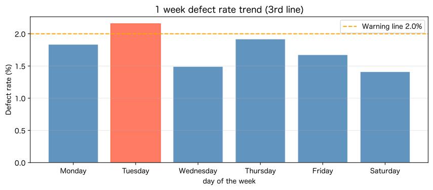

Step 3: Graph output completed

Reading the results

From the graph, Tuesday (2.16%) is above the warning line (2.0%). You can see it visually (red bar).
Thursday (1.92%) is just below the warning line and should be monitored for risks.

The advantage of “separating cells” is when you want to modify this graph. You only need to rewrite cell 3.
Modifications are safer and faster because you don’t have to touch the data definition (cell 1) or aggregation (cell 2).

Organizational benefits: Cell division has the effect of “turning code into a natural procedure manual”.
The entire Jupyter Notebook can be used as a transfer document.

---

No.010: Understand the basic flow of data analysis

Practical meaning

Learning the flow of data analysis is the core of promoting DX in the manufacturing industry.
Once you are able to answer the question “I have data → how should I analyze it?” You will be able to convert on-site issues into a form that can be solved using data.

Concept of analysis and modeling

Data analysis in the manufacturing industry will be easier to organize if you think about it along the lines of CRISP-DM.

1. Business understanding: Define what you want to solve
       ↓
2. Data understanding: Understand the quantity, quality, and structure of the data at hand
       ↓
3. Data preparation: Perform missing/outlier/type conversion/combining
       ↓
4. Modeling: Apply aggregation, statistics, and machine learning models
       ↓
5. Evaluation: Check whether the results are useful for on-site issues
       ↓
6. Deployment: Incorporate into regular reports, dashboards, and automatic notifications

This time, we will use everything we learned in No.001~009, Create a Mini Analysis Report to analyze the fictitious 3rd line 2024 Q1 data.

Check with Python

# No.010 - Step 1: Confirm the data (the fictitious data has been created at the beginning)

print("=== Step 1: Check data ===")
print(f"  period       : 2024yearQ1({n_days}days)")
print(f"  Total production number   : {production.sum():>8,} stand")
print(f"  Total number of defective items : {defects.sum():>8,} units")
print(f"  Average defect rate : {defect_rate_pct.mean():>8.2f} %")
print(f"  Average occupancy rate : {operation_rate.mean():>8.1f} %")
print()

# Check basic statistics
print(f"{'indicators':<16} {'Production quantity (units)':>12} {'Defect rate (%)':>12} {'Occupancy rate (%)':>12}")
print("-" * 55)
stats_rows = [
    ("maximum value", production.max(), defect_rate_pct.max(), operation_rate.max()),
    ("minimum value", production.min(), defect_rate_pct.min(), operation_rate.min()),
    ("average value", production.mean(), defect_rate_pct.mean(), operation_rate.mean()),
    ("standard deviation", production.std(), defect_rate_pct.std(), operation_rate.std()),
]
for label, p, d, o in stats_rows:
    print(f"{label:<16} {p:>12.1f} {d:>12.2f} {o:>12.2f}")

=== Step 1: Check data === Period: Q1 2024 (90 days) Total production: 89,243 units Total number of defective items: 1,799 pieces Average defect rate: 2.01% Average occupancy rate: 94.0%

Indicator Production quantity (units) Defect rate (%) Operation rate (%)
----------------------------------------------------------
Maximum value 1148.0 3.22 99.00
Minimum value 790.0 0.85 88.93
Average value 991.6 2.01 93.98
Standard deviation 74.4 0.59 2.05

# No.010 - Step 2: Monthly tally of defect rate and operating rate

# Monthly slice (January: 0-30, February: 31-58, March: 59-89)
monthly_splits = [(0, 31, "January"), (31, 59, "February"), (59, 90, "March")]

# Number of days above warning line
high_defect_days = int((defect_rate_pct >= 2.0).sum())
alert_days = int((defect_rate_pct >= 3.0).sum())

print("=== Step 2: Aggregation of defect rate ===")
print(f"  Warning line (2%or more) Excess: {high_defect_days:>3} days / {n_days} during the day ({high_defect_days/n_days*100:.1f}%)")
print(f"  Alert line (3%above): {alert_days:>3} days / {n_days} during the day ({alert_days/n_days*100:.1f}%)")
print()

print(f"{'moon':<6} {'Production number':>10} {'Number of defective products':>10} {'Defect rate':>10} {'occupancy rate':>10}")
print("-" * 50)
for s, e, label in monthly_splits:
    mp = production[s:e].sum()
    md_val = defects[s:e].sum()
    mr = md_val / mp * 100
    mo = operation_rate[s:e].mean()
    print(f"{label:<6} {mp:>10,} {md_val:>10,} {mr:>9.2f}% {mo:>9.1f}%")

=== Step 2: Aggregation of defect rate === Warning line (2% or more) exceeded: 49 days / 90 days (54.4%) Alert line (3% or more): 2 days / 90 days (2.2%)

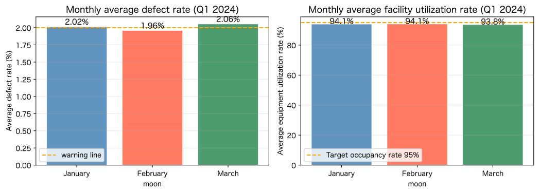
Month Production quantity Number of defective items Defect rate Operation rate
--------------------------------------------------
January 30,484 617 2.02% 94.1%
February 27,663 541 1.96% 94.1%
March 31,096 641 2.06% 93.8%

# No.010 - Step 3: Time series graph (3 panels)

fig, axes = plt.subplots(3, 1, figsize=(12, 11))

# ---- Graph 1: Trends in daily production ----
axes[0].plot(day_index, production, color="steelblue", linewidth=1.5, alpha=0.85, label="Actual production number")
axes[0].axhline(y=1000, color="crimson", linestyle="--", linewidth=1.5, label="Target (1,000 units)")
axes[0].fill_between(
    day_index, production, 1000, where=(production < 1000), alpha=0.15, color="crimson", label="Goal unachieved zone"
)
axes[0].set_title("Trends in daily production (Q1 2024 / 3rd line)", fontsize=13)
axes[0].set_xlabel("Number of days elapsed (days)")
axes[0].set_ylabel("Production quantity (units)")
axes[0].legend(fontsize=10)
axes[0].grid(True, alpha=0.3)

# ---- Graph 2: Trends in defect rate ----
axes[1].plot(day_index, defect_rate_pct, color="tomato", linewidth=1.5, alpha=0.85)
axes[1].axhline(y=2.0, color="orange", linestyle="--", linewidth=1.5, label="Warning line 2.0%")
axes[1].axhline(y=3.0, color="crimson", linestyle="--", linewidth=1.5, label="Alert line 3.0%")
axes[1].fill_between(
    day_index, defect_rate_pct, 3.0, where=(defect_rate_pct > 3.0), alpha=0.2, color="crimson", label="alert zone"
)
axes[1].set_title("Daily defect rate trends (2024 Q1/3rd line)", fontsize=13)
axes[1].set_xlabel("Number of days elapsed (days)")
axes[1].set_ylabel("Defect rate (%)")
axes[1].legend(fontsize=10)
axes[1].grid(True, alpha=0.3)

# ---- Graph 3: Distribution of equipment utilization rate (histogram) ----
axes[2].hist(operation_rate, bins=20, color="seagreen", edgecolor="white", alpha=0.85)
axes[2].axvline(
    x=float(operation_rate.mean()),
    color="crimson",
    linestyle="--",
    linewidth=1.5,
    label=f"average value: {operation_rate.mean():.1f}%",
)
axes[2].axvline(x=95.0, color="orange", linestyle=":", linewidth=1.5, label="Target occupancy rate: 95%")
axes[2].set_title("Distribution of equipment utilization rate (2024 Q1 / 3rd line)", fontsize=13)
axes[2].set_xlabel("Equipment utilization rate (%)")
axes[2].set_ylabel("Number of days (days)")
axes[2].legend(fontsize=10)
axes[2].grid(True, alpha=0.3)

plt.tight_layout()
plt.show()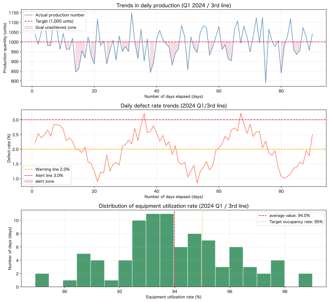

# No.010 - Step 4: Monthly comparison graph

months = ["January", "February", "March"]
splits = [(0, 31), (31, 59), (59, 90)]
monthly_defect_rate_avg = [defect_rate_pct[s:e].mean() for s, e in splits]
monthly_op_rate_avg = [operation_rate[s:e].mean() for s, e in splits]
bar_colors = ["steelblue", "tomato", "seagreen"]

fig, axes = plt.subplots(1, 2, figsize=(11, 4))

# Monthly average defect rate
axes[0].bar(months, monthly_defect_rate_avg, color=bar_colors, edgecolor="white", alpha=0.85)
axes[0].axhline(y=2.0, color="orange", linestyle="--", linewidth=1.5, label="warning line")
for i, v in enumerate(monthly_defect_rate_avg):
    axes[0].text(i, v + 0.03, f"{v:.2f}%", ha="center", fontsize=11, fontweight="bold")
axes[0].set_title("Monthly average defect rate (Q1 2024)", fontsize=13)
axes[0].set_xlabel("moon")
axes[0].set_ylabel("Average defect rate (%)")
axes[0].legend()
axes[0].grid(True, axis="y", alpha=0.3)

# Monthly average capacity utilization rate
axes[1].bar(months, monthly_op_rate_avg, color=bar_colors, edgecolor="white", alpha=0.85)
axes[1].axhline(y=95.0, color="orange", linestyle="--", linewidth=1.5, label="Target occupancy rate 95%")
for i, v in enumerate(monthly_op_rate_avg):
    axes[1].text(i, v + 0.05, f"{v:.1f}%", ha="center", fontsize=11, fontweight="bold")
axes[1].set_title("Monthly average facility utilization rate (Q1 2024)", fontsize=13)
axes[1].set_xlabel("moon")
axes[1].set_ylabel("Average equipment utilization rate (%)")
axes[1].legend()
axes[1].grid(True, axis="y", alpha=0.3)

plt.tight_layout()
plt.show()

findfont: Failed to find font weight bold, now using 400.

Reading the results

The following findings can be read from the graph.

① Changes in production volume (Graph 1) Approximately 40% of the days the number of units fell below the target of 1,000 units.
There is no concentration in a specific period, and we see intermittent production fluctuations throughout the line.
It is necessary to check these fluctuation factors (setup changes, material waiting, malfunction stoppages) with records.

② Trend of defect rate (Graph 2/Monthly bar graph) The defect rate fluctuates periodically within the month (low at the beginning of the month and high in the middle), The influence of specific process conditions (raw material lot change, tool wear) is suspected.
By month, March (2.06%) and January (2.02%) exceeded the warning line. February (1.96%) is the lowest. If March levels continue after Q2, countermeasures will be necessary.

③ Distribution of equipment utilization rate (Graph 3/Monthly bar graph) The average equipment utilization rate was 94.0%, falling short of the target (95%).
The tail of the distribution has widened to the 88% level, and sudden equipment outages are occurring sporadically.
By month, March (93.8%) was the lowest, indicating a decline in the occupancy rate in the second half of Q1.
A review of the maintenance plan for April is required.

---

Overall Suggestions: By automatically running this kind of analysis every month, you can detect problems early. Enables quick reporting to administrators.
Using Python, you only have to write this series of analysis code once. You can “replace only the data and run” every month.

---

Practical implications seen through target exerciseing

Through No.001 to No.010, the following points were demonstrated in practical terms.

1. “Introduction” is directly connected to issues at the manufacturing site

print Even if you have basic knowledge such as sentences and comments, Production status log output'' and Code transfer document creation” It can be converted into concrete business value.

2. Errors are not “walls” but “information”

ZeroDivisionError and NameError are It tells you about “holidays”, “missing values”, and “type mismatch” in manufacturing data.
The habit of reading errors will directly lead to improved data quality.

3. Cell division is “documentation of analysis flow”

Dividing code into cells is synonymous with “automatically generating an analysis procedure manual.”
Jupyter Notebook can be used as is as a handover document/report.

4. You can see the “overall picture of analysis” with 10 books

Analysis flow of No.010 (Collection → Confirmation → Aggregation → Visualization) By experiencing it repeatedly, the learning from Chapter 2 onwards will become much easier to understand.

What you need to implement in practice

In order to implement the contents of Chapter 1 into the actual manufacturing site, the following steps are required.

Step 1: Prepare the environment

Work	Contents
Installing Python	Anaconda or pyenv + venv
Introduction to Jupyter	pip install jupyter or JupyterLab
Unify libraries	Align your team environment with requirements.txt
Check execution privileges	Check company security policy (especially in Windows environment)

Step 2: Connect with existing data

• Load Excel file: openpyxl (explained in Chapters 6-8)
• CSV loading: csv module, polars
• Database connection: sqlalchemy, pyodbc

Step 3: Design the analysis cycle

It is important to create a system for regular execution and regular reporting, rather than “analyzing only once”.
Start with simple aggregation and visualization, A realistic roadmap is to step up to prediction/machine learning after seeing the results.

Step 4: Knowledge sharing within the organization

• Manage analysis code with Git (GitHub, GitLab)
• Create rules to share Jupyter Notebooks within your team
• Maintain an environment where “anyone can run code written by someone”

Summary

In this article, Python 100 Exercises Chapter 1 (No.001 to No.010) Introduction to Python based on production line operating data explained.

Review of what you learned

No.	Title	Key points for use in the manufacturing industry
001	Understand what you can do with Python	Understand the overall picture of DX
002	Why Python is used for data analysis	Organizing the basis for tool selection
003	Prepare the execution environment	Unify the environment as a team
004	Basic operations of Jupyter Notebook	Use for automatic generation of analysis reports
005	Executing scripts	Creating a foundation for regular execution and automation
006	Displaying characters with the print function	Used for log output and status confirmation
007	Write a comment	Leave code inheritance materials
008	How to read error displays	Detect data quality problems early
009	Execute code cells separately	Design analysis flow step by step
010	Basic flow of data analysis	Q1 Experience the overall analysis of production results

Next steps

Chapter 2 (No.011 to 020) describes the methods often used in calculations at manufacturing sites. Learn “variables, types, and operations.” Calculation of unit price, quantity, yield rate, etc. Master the numerical processing required in the field using Python.

Consultation for corporations

---

Surikobo provides Python training and data analysis support for manufacturing industry and DX promotion staff.

Do you have any of these problems?

• “I want to put the contents of this chapter into practice using my own manufacturing data.”
• “I would like you to create customized Python training for our company.”
• “I want to migrate Excel management to Python”
• “I want to develop a data analysis platform for quality control and production management”

Services provided

Service	Overview
Python training for the manufacturing industry	Practical training using field data (online/face-to-face)
Data analysis infrastructure construction support	Integrated management system design for production, quality, and cost data
KPI dashboard development	Real-time manufacturing index visualization tool development
DX promotion consulting	Consistent support from problem organization to implementation

---

📩 Contact: surikobo.co.jp/contact Please feel free to contact us first.