Process quality data on the manufacturing line in bulk at high speed with NumPy

100 Exercises Chapter 7 (No.061-No.070): Introduction to NumPy

This article is Chapter 7 of the “100 Exercises on Introduction to Python for Data Analysis” series.
In Chapter 6 (No.051-060), we learned file operations and CSV.
In this chapter, we will use NumPy to collect quality data (90 days, 3 lines) of a precision machinery parts factory. Learn how to work with Python lists faster and more concisely.

[!NOTE] This material is a notebook that has been used in corporate training by Surikobo (or its representative, Hiroshi Wayama) in the past, and has been reorganized and edited with the permission of the company and published.
All published data is fictitious and has no relation to actual companies, factories, or numbers.

Introduction: Practical issues in the manufacturing industry covered in this article

This is a problem faced by Mr. K, who is in charge of data analysis at a precision machinery parts factory.

Current situation
  1. Daily production numbers and defective numbers for 3 lines are accumulated in 90 days x 3 sheets.
  2. Because a for loop is written to calculate the defect rate, the code is long and difficult to maintain.
  3. Every time you answer the question, “When was the day last month when the defect rate was the highest?”
     Searching for 270 numbers manually
  4. Calculate statistics individually in Excel to evaluate stability (variation) for each line

Using NumPy, you can calculate the defect rate of 270 items (3 lines x 90 days) in 1 line, Find the maximum value, minimum value, average, and standard deviation using one function, You can instantly extract the warning date (defect rate > threshold) using fancy index.

Common situations in the field

Scene	Task
Batch calculation of defect rate	for Process 90 rows sequentially in a loop. The code is long and slow as the number of lines increases
Average by month and line	Apply Excel’s AVERAGE function to each column and sheet individually
Extracting abnormal values (warning days)	Manually filtering “days with defect rate > 2%”, there is a risk of oversight
Stability evaluation	Calculate the standard deviation of each line individually and calculate the coefficient of variation (CV) by hand
Horizontal comparison of multiple lines	Files are separated for each line, making it difficult to grasp the overall picture

NumPy’s Vector operations, Boolean index, Aggregation functions (axis specification) When combined, these tasks can be automated with just a few lines of code.

Why is this problem difficult to judge?

Although NumPy appears to have low learning costs, it has the following pitfalls when working with manufacturing data:

1. axis orientation confusion In a two-dimensional array, np.mean(data, axis=0) is the average in the column direction (daily), axis=1 is the “row direction (by line)” average.
   Check shape first and understand which is the row and which is the column before operating it.

2. Slice returns view The slice of sub = array[10:20] is a reference, not a copy.
   If you set sub[0] = 99, the original array will also change.
   Specify .copy() to prevent unintended changes

3. dtype pitfalls int32 Division between arrays results in float, but Please be aware that truncation occurs in integer operations (// and %)

4. Boolean index returns copy In-place assignment of array[array > 2.0] = 0 changes the original array, but sub = array[array > 2.0] returns a new copy.
   Be careful because the behavior is different between assignment and reference.

Overall picture of the exercises covered in this chapter

No.	Title	Usage in manufacturing industry
061	Understanding the role of NumPy	Comparing the speed and simplicity of Python list vs. NumPy
062	Import NumPy	Check import and frequently used functions
063	Create a NumPy array	Array the daily production number, defective number, and dimension measurements
064	Check the array shape	Understand the structure of two-dimensional data with shape / ndim / dtype / size
065	Extracting elements of an array	Extracting a specific date or line using index, slice, or 2-dimensional access
066	Batch calculation for arrays	Simultaneous calculation of defect rate, sales, and loss for 270 items (broadcast)
067	Calculate the average value	axis Batch calculation and bar graph visualization of average defect rate by line and month
068	Calculate maximum and minimum values	Identify worst and best days with argmax / argmin
069	Calculate standard deviation	Horizontal comparison of line quality stability using coefficient of variation (CV)
070	Extract data that meets the conditions	Automatically extract warning dates with np.where and visualize with scatter plot

Preparing the Python environment

import subprocess, sys
res = subprocess.run(["sw_vers", "-productVersion"], capture_output=True, text=True)
print(f"macOS : {res.stdout.strip()}")
print(f"Python: {sys.version}")

macOS : 26.3
Python: 3.13.1 (main, Dec  3 2024, 17:59:52) [Clang 16.0.0 (clang-1600.0.26.4)]

import numpy as np
import matplotlib
import matplotlib.pyplot as plt
import matplotlib.ticker as ticker
import datetime

matplotlib.rcParams['font.family'] = 'Hiragino Maru Gothic Pro'
%config InlineBackend.figure_format = 'svg'
np.random.seed(42)

print("Library loading completed")
print(f"  NumPy     : {np.__version__}")
print(f"  Matplotlib: {matplotlib.__version__}")

Library loading completed NumPy: 2.5.1 Matplotlib: 3.11.0

Creation of fictitious data

Assumed scenario: Precision mechanical parts factory / machining line quality control team Period: January 1, 2024 - March 30, 2024 (90 days) Management target: 3 product lines (precision shafts, bearings, flanges) Data format: 2D NumPy array — shape: (3, 90) = (number of lines, number of days)

np.random.seed(42)

# ── Basic settings ────────────────────────────────────────────
lines        = ["M1-Precision axis", "M2-Bearing", "M3-flange"]
unit_prices  = np.array([2400, 1800, 1200])   # yen/piece
n_days       = 90                              # 2024-01-01~03-30
base_date    = datetime.date(2024, 1, 1)

# Month index (0=January: 31 days, 1=February: 29 days, 2=March: 30 days)
month_idx = np.array([0]*31 + [1]*29 + [2]*30, dtype=np.int32)

# ── Daily production number (3 lines x 90 days) ──────────────────────────
base_prod = [450, 380, 550]
prod_2d = np.array([
    np.random.randint(b - 20, b + 21, size=n_days)
    for b in base_prod
], dtype=np.int32)   # shape: (3, 90)

# ── Daily defective number ──────────────────────────────────────────
dr_base = [0.018, 0.022, 0.014]
defect_2d = np.array([
    np.maximum(1, np.round(
        prod_2d[i] * dr_base[i] + np.random.randn(n_days) * 1.2
    ).astype(int))
    for i in range(3)
], dtype=np.int32)   # shape: (3, 90)

# ── Daily defect rate ──────────────────────────────────────────
defect_rates_2d = defect_2d / prod_2d * 100  # shape: (3, 90), dtype: float64

# ── Confirmation display ────────────────────────────────────────────
print(f"array size: prod_2d{prod_2d.shape}, defect_2d{defect_2d.shape}, "
      f"defect_rates_2d{defect_rates_2d.shape}")
print()
print(f"{'line':<14} {'Weekly total (production)':>10} {'Weekly total (bad)':>10} {'Average defect rate':>10} {'Maximum defect rate':>10}")
print("=" * 58)
for i, line in enumerate(lines):
    print(f"{line:<14} {int(prod_2d[i].sum()):>10,} {int(defect_2d[i].sum()):>10} "
          f"{float(defect_rates_2d[i].mean()):>9.2f}% {float(defect_rates_2d[i].max()):>9.2f}%")

Array size: prod_2d(3, 90), defect_2d(3, 90), defect_rates_2d(3, 90)

Line Weekly total (production) Weekly total (defective) Average defect rate Maximum defect rate
===========================================================
M1-Precision shaft 40,387 745 1.84% 2.55%
M2-Bearing 34,339 771 2.24% 2.89%
M3-Flange 49,581 711 1.43% 1.94%

---

No.061: Understand the role of NumPy

Practical meaning

When calculating the daily defect rate of a production line, the Python for loop 90 loops are required. Using NumPy’s vector operations, The same calculation is completed by applying to one row/entire array.
Even if the data increases to 10,000 rows or 10 lines, the NumPy code will not change.

Concept of analysis and modeling

NumPy internally performs array operations implemented in C language, so 10-100x faster than Python’s for loop.
Numerical calculation libraries (pandas, scikit-learn, scipy) use NumPy internally. Understanding NumPy’s array operations is the foundation for advanced data analysis.

Check with Python

# Comparing the simplicity of Python lists (for loops) and NumPy

production_list = list(prod_2d[0])     # 90 days of M1
defect_list     = list(defect_2d[0])

# ── Pure Python: Calculate defect rate with for loop ────────────────
defect_rates_py = []
for prod, def_count in zip(production_list, defect_list):
    defect_rates_py.append(def_count / prod * 100)
mean_py = sum(defect_rates_py) / len(defect_rates_py)

# ── NumPy: 1 line in vector operation ──────────────────────────────
defect_rates_np = defect_2d[0] / prod_2d[0] * 100
mean_np = defect_rates_np.mean()

print("=== Comparison of calculation results (M1-Precision axis, 90 days) ===")
print(f"  Python top of list5records: {[round(r, 2) for r in defect_rates_py[:5]]}")
print(f"  NumPy array  top5records: {defect_rates_np[:5].round(2)}")
print()
print(f"  Python average: {mean_py:.4f}%")
print(f"  NumPy average : {mean_np:.4f}%   (No error)")
print()
print("=== Code difference ===")
print("Python: for loop 4 lines + sum/len")
print("NumPy : defect_2d[0] / prod_2d[0] * 100 ← Completed in one line")
print()
print(f"  Difference in type: Python={type(defect_rates_py).__name__}, NumPy={type(defect_rates_np).__name__}")
print(f"  NumPy dtype: {defect_rates_np.dtype}")

=== Comparison of calculation results (M1-Precision axis, 90 days) === Python Top 5 items in list: [np.float64(1.71), np.float64(1.53), np.float64(2.03), np.float64(2.06), np.float64(2.0)] NumPy array First 5 items: [1.71 1.53 2.03 2.06 2. ]

  Python average: 1.8439%
  NumPy average: 1.8439% (no error)

=== Code difference ===
  Python: for loop 4 lines + sum/len
  NumPy : defect_2d[0] / prod_2d[0] * 100 ← Completed in one line

  Type difference: Python=list, NumPy=ndarray
  NumPy dtype: float64

Reading the results

The calculation results for the Python list and NumPy array are completely consistent.
90 defect rates were calculated for one line of defect_2d[0] / prod_2d[0] * 100.
This is NumPy’s vector operations.
Even if the number of data items increases from 90 items to 9,000 items to 900,000 items, the NumPy code does not change.
You can write highly maintainable code even as manufacturing data increases.

---

No.062: Import NumPy

Practical meaning

import numpy as np is the standard NumPy import method.
The np alias is an industry standard and is used by other libraries as well. It is designed to expect NumPy arrays as input.

Concept of analysis and modeling

NumPy is the cornerstone of the data analytics ecosystem.
pandas’ Series / DataFrame is built on top of NumPy arrays, The input to the scikit-learn model also uses NumPy arrays.
Learning the basics of NumPy will ease the transition to more advanced libraries.

Check with Python

import numpy as np

print(f"NumPy version: {np.__version__}")
print()

# NumPy functions commonly used in manufacturing data analysis
kpi_funcs = [
    ("np.array()",        "List → array conversion"),
    ("np.zeros(n)",       "Initializing zero arrays (alert flags, etc.)"),
    ("np.arange(n)",      "Sequential number array (generate daily index)"),
    ("np.mean()",         "Average value (monthly average of defect rate)"),
    ("np.std()",          "Standard deviation (quality stability evaluation)"),
    ("np.max() / min()",  "Maximum/Minimum (worst day/best day)"),
    ("np.argmax()",       "Maximum value index (day)"),
    ("np.where()",        "Extraction/labeling based on conditions"),
    ("np.sum(axis=)",     "Total (accumulated by row/column by specifying axis)"),
    ("np.cumsum()",       "Cumulative sum (monthly cumulative production number)"),
]
print(f"{'function':<28} {'Utilization in manufacturing data'}")
print("=" * 68)
for fname, desc in kpi_funcs:
    print(f"  {fname:<26} {desc}")

print()
# NumPy constants
print(f"np.pi  = {np.pi:.6f}   (Circumference and area calculation of circular parts)")
print(f"np.inf = {np.inf}       (as an initial value with no upper limit)")
print(f"np.nan = {np.nan}       (Representation of missing values)")

NumPy version: 2.5.1

Functions Utilization in manufacturing data
====================================================================
  np.array() List → array conversion
  np.zeros(n) Initialize zero array (alert flags, etc.)
  np.arange(n) Sequential number array (generates daily index)
  np.mean() Average value (monthly average of defect rate)
  np.std() Standard deviation (quality stability evaluation)
  np.max() / min() Maximum/minimum (worst day/best day)
  np.argmax() Maximum value index (day)
  np.where() Extraction/labeling based on conditions
  np.sum(axis=) Total (accumulate by row/column by specifying axis)
  np.cumsum() Cumulative sum (monthly cumulative production number)

np.pi = 3.141593 (calculation of circumference and area of circular parts)
np.inf = inf (as an initial value with no upper limit)
np.nan = nan (missing value representation)

Reading the results

The four most commonly used in manufacturing data analysis are np.mean, np.std, np.argmax, and np.where.
np.inf is used in the algorithm to find the minimum value as an initial value with no upper limit.
np.nan is used to express missing values ​​(sensor stopped/recording failure).
For arrays containing np.nan, np.mean returns nan, so If there are missing values, use np.nanmean/np.nanstd.

---

No.063: Create NumPy array

Practical meaning

Learn how to create manufacturing data as a NumPy array.
Data read from CSV or Excel is ultimately converted to a NumPy array for processing.
If you use np.random.normal(), you can also use simulation data of dimension measurements. It can be generated in a form close to reality.

Concept of analysis and modeling

There are four main ways to create NumPy arrays.
① Convert from list with np.array(), ② Initialize with np.zeros/ones(), ③ np.arange/linspace() is an equally spaced sequence, ④ np.random.*() is random data.
Dimensional measurements at manufacturing sites often follow a normal distribution $N(\mu, \sigma^2)$. np.random.normal(mean, std, size) allows for faithful simulation.

Check with Python

# 4 ways to create NumPy arrays

# 1. Convert from list with np.array()
weekly_prod_063 = np.array([450, 462, 438, 471, 445, 457, 448])
print(f"1. np.array() : {weekly_prod_063}  shape={weekly_prod_063.shape}")

# 2. Initialize with np.zeros() (alert flags, etc.)
alert_flags = np.zeros(n_days, dtype=np.int8)
print(f"2. np.zeros() : {alert_flags[:5]} ...  shape={alert_flags.shape}, dtype={alert_flags.dtype}")

# 3. Sequential numbers with np.arange()
day_indices = np.arange(n_days)           # 0~89
print(f"3. np.arange(): {day_indices[:7]} ...  shape={day_indices.shape}")

# 4. Generate dimension measurements with np.random.normal() (shaft diameter inspection of precision shaft)
target_diam  = 25.000   # Target diameter mm
tolerance    = 0.050    # Tolerance ±0.05mm
sigma_diam   = tolerance / 3   # 3σ = Tolerance full width → σ = 0.0167mm
measurements = np.random.normal(target_diam, sigma_diam, size=30)

print()
print("=== M1-Precision shaft shaft diameter measurement (n=30 samples) ===")
print(f"  Target value   : {target_diam:.3f} mm  Tolerance: ±{tolerance:.3f} mm")
print(f"  top5records  : {measurements[:5].round(4)} mm")
print(f"  average     : {measurements.mean():.4f} mm")
print(f"  range     : {measurements.min():.4f} ~ {measurements.max():.4f} mm")
print()

# Specifying dtype
arr_int   = np.array([1.7, 2.3, 3.9], dtype=np.int32)   # round down decimal
arr_float = np.array([1, 2, 3],        dtype=np.float64)
print(f"dtype=int32  conversion: {arr_int}   (decimals are rounded down)")
print(f"dtype=float64conversion: {arr_float}")

1. np.array() : [450 462 438 471 445 457 448] shape=(7,) 2. np.zeros() : [0 0 0 0 0] … shape=(90,), dtype=int8 3. np.arange(): [0 1 2 3 4 5 6] … shape=(90,)

   === M1-Precision shaft shaft diameter measurement (n=30 samples) === Target value: 25.000 mm Tolerance: ±0.050 mm First 5 items: [25.0187 24.976 24.998 24.9987 24.9816] mm Average: 24.9983 mm Range: 24.9620~25.0396mm

   dtype=int32 conversion: [1 2 3] (round down decimals) dtype=float64 conversion: [1. 2. 3.]

Reading the results

np.random.normal(25.000, 0.0167, size=30) simulated normal distribution measurements of shaft diameter.
Because we use “3σ = total tolerance width (0.1mm)” as the tolerance design, Compatible with “±3σ management” in quality engineering.
Theoretically, 99.73% of products fall within tolerance.
When dtype=np.int32 converts float, decimals are truncated.
The behavior is the same as the int() function, but NumPy’s strength is that it can be applied to the entire array at once.

---

No.064: Check the shape of the array

Practical meaning

When handling manufacturing data as a two-dimensional array (matrix), Whether the rows are lines and the columns are dates or the rows are dates and columns are lines. It is important to check shape before operating.
If the direction of the axis is incorrect, the results of averaging and aggregation will be completely reversed.

Concept of analysis and modeling

The four attributes shape, ndim, dtype, and size are the “addresses” of the NumPy array.
If you have the habit of adding one line print(array.shape) before array operations, Most of the bugs caused by misdirection in axis can be prevented.

Check with Python

# Understand the structure of an array using shape / ndim / dtype / size

print("=== 1-dimensional array (M1 daily production quantity) ===")
a1 = prod_2d[0]                           # shape: (90,)
print(f"  shape: {a1.shape}  → {a1.shape[0]} days")
print(f"  ndim : {a1.ndim}     → 1dimension")
print(f"  dtype: {a1.dtype} → integer type")
print(f"  size : {a1.size}    → Number of elements")
print()

print("=== 2D array (all lines x all days) ===")
print(f"  shape: {prod_2d.shape}")
print(f"    → rows = {prod_2d.shape[0]}Line (M1, M2, M3)")
print(f"    → columns = {prod_2d.shape[1]}day (2024-01-01~03-30)")
print(f"  ndim : {prod_2d.ndim}     → 2dimension")
print(f"  dtype: {prod_2d.dtype}")
print(f"  size : {prod_2d.size}    → Total number of elements ({prod_2d.shape[0]} × {prod_2d.shape[1]})")
print()

print("=== Defect rate array (float64) ===")
print(f"  shape: {defect_rates_2d.shape}, dtype: {defect_rates_2d.dtype}")
print()

# Check axis using shape
print("=== Difference between axis=0 vs axis=1 (check with np.sum) ===")
sum_axis0 = prod_2d.sum(axis=0)   # Total of all lines for each day → shape: (90,)
sum_axis1 = prod_2d.sum(axis=1)   # All-day total for each line → shape: (3,)
print(f"  axis=0(column direction, total by day): shape={sum_axis0.shape}  top3days={sum_axis0[:3]}")
print(f"  axis=1(Row direction, line total): shape={sum_axis1.shape}  value={sum_axis1}")
print()
for i, line in enumerate(lines):
    print(f"  {line} 90Total daily production: {int(sum_axis1[i]):,} units")

=== 1-dimensional array (M1 daily production quantity) === shape: (90,) → 90 days ndim : 1 → 1-dimensional dtype: int32 → integer type size : 90 → number of elements

=== 2D array (all lines x all days) ===
  shape: (3, 90)
    → row = 3 lines (M1, M2, M3)
    → Column = 90 days (2024-01-01~03-30)
  ndim : 2 → 2D
  dtype: int32
  size: 270 → total number of elements (3 × 90)

=== Defect rate array (float64) ===
  shape: (3, 90), dtype: float64

=== Difference between axis=0 vs axis=1 (check with np.sum) ===
  axis=0 (column direction, total by day): shape=(90,) First 3 days=[1414 1416 1369]
  axis=1 (row direction, line total): shape=(3,) value=[40387 34339 49581]

  M1-Precision axis 90 days total production: 40,387 pieces
  M2-bearing 90 days total production: 34,339 pieces
  M3-Flange 90 days total production: 49,581 pieces

Reading the results

You can check “row = 3 lines, column = 90 days” from prod_2d.shape = (3, 90).
axis=0 is row-oriented (aggregation across columns), so “total of all lines for each day”, axis=1 is column-oriented (aggregation across rows), so it is the “all-day total for each line”.
np.mean(prod_2d, axis=1) allows you to calculate the “average daily production number by line”.
It is important to always check shape and be aware of the direction of axis before operation.

---

No.065: Extract elements of array

Practical meaning

“Extract only the data for the second week of the M2 line” “Compare the data for January 1st for all lines” Such access to specific dates and specific lines is routinely required for manufacturing data analysis.
NumPy’s indexing and slicing allows us to write this concisely.

Concept of analysis and modeling

NumPy’s slice returns a view. If you need a copy, use .copy().
Fancy indexing (indexing by integer array/Boolean array) returns a copy.
Being aware of which one you are using when processing data is the key to preventing bugs.

Check with Python

# Extract elements using index, slice, and 2D access

prod_m1 = prod_2d[0]   # M1 line, shape: (90,)

print("=== 1D index access ===")
print(f"  first day [0]    : {prod_m1[0]:,} units")
print(f"  last days [-1]   : {prod_m1[-1]:,} units")
print(f"  10day [9]  : {prod_m1[9]:,} units")
print()

print("=== Slice by week ===")
week1 = prod_m1[:7]    # Week 1 (1/1-1/7)
week2 = prod_m1[7:14]  # Week 2 (1/8-1/14)
print(f"  No.1week ( 1/ 1~ 1/ 7): {week1}  Total={int(week1.sum()):,}units")
print(f"  No.2week ( 1/ 8~ 1/14): {week2}  Total={int(week2.sum()):,}units")
print()

print("=== 2D array access ===")
print(f"  M1 of1day   prod_2d[0, 0]   = {prod_2d[0, 0]:,} units")
print(f"  M2 of1day   prod_2d[1, 0]   = {prod_2d[1, 0]:,} units")
print(f"  of all lines1day prod_2d[:, 0] = {prod_2d[:, 0]}  (Number of production for each line)")
print(f"  M3 all of90days  prod_2d[2, :].shape = {prod_2d[2, :].shape}")
print()

print("=== Copy the slice with view → .copy() ===")
sub = prod_m1[10:15].copy()   # get a copy
original_val = prod_m1[10]
sub[0] = 9999
print(f"  sub[0] The 9999 changed to → original array prod_m1[10] = {prod_m1[10]}  (No change)")

=== 1D index access === First day [0]: 468 pieces Last day [-1]: 464 pieces Day 10 [9]: 440 pieces

=== Slice by week ===
  Week 1 (1/1 to 1/7): [468 458 444 437 450 468 448] Total = 3,173 pieces
  2nd week (1/8 - 1/14): [452 440 440 453 465 469 453] Total = 3,172 pieces

=== 2D array access ===
  M1 day 1 prod_2d[0, 0] = 468 pieces
  M2 day 1 prod_2d[1, 0] = 394 pieces
  Day 1 of all lines prod_2d[:, 0] = [468 394 552] (number of production for each line)
  All 90 days of M3 prod_2d[2, :].shape = (90,)

=== Copy the slice with view → .copy() ===
  Change sub[0] to 9999 → Original array prod_m1[10] = 453 (no change)

Reading the results

prod_2d[:, 0] is a slice called “Day 1 (column 0) of all lines”, The daily production numbers for all three lines are collected together.
By creating a copy with .copy(), we were able to prevent the original array from being affected.
Even after setting sub[0] = 9999, the value of prod_m1[10] has not changed. You can confirm that the copy is working properly.

---

No.066: Batch calculation for arrays

Practical meaning

NumPy’s broadcast feature allows arrays of different shapes to You can automatically match the shapes and perform calculations.
If you transform unit_prices (form (3,)) to (3, 1), Multiply by the production number array of (3, 90), Sales for all lines and all days can be calculated at once without loops.

Concept of analysis and modeling

Broadcast rules: When operating on two arrays of different shapes, If each dimension is “either the same or 1”, the dimension with shape 1 will be automatically expanded.
The conversion (3,1) × (3,90) → (3,90) will be performed automatically.

Check with Python

# Calculate 270 KPIs at once using vector operations and broadcasting

# Number of good products (vector subtraction)
good_units_2d = prod_2d - defect_2d          # shape: (3, 90)

# Sales (broadcast: transformed to unit_prices (3,) → (3,1))
revenue_2d = good_units_2d * unit_prices.reshape(3, 1)  # shape: (3, 90)

# Loss (number of defects × unit price × (1 + disposal cost rate))
penalty = 0.30
loss_2d = defect_2d * unit_prices.reshape(3, 1) * (1 + penalty)   # shape: (3, 90)

print("=== Vector operation result (first 3 days of each line) ===")
print(f"{'line':<14} {'days':>4} {'production':>6} {'defective':>5} {'Defect rate (%)':>10} {'Good product sales':>12} {'defect loss':>10}")
print("-" * 66)
for i, line in enumerate(lines):
    for j in range(3):
        dr = float(defect_rates_2d[i, j])
        print(f"{line if j==0 else '':<14} {j+1:>4} {int(prod_2d[i,j]):>6,} "
              f"{int(defect_2d[i,j]):>5} {dr:>9.2f}% "
              f"{int(revenue_2d[i,j]):>12,} {int(loss_2d[i,j]):>10,}")

print()
print("=== Weekly aggregation (slice + sum) ===")
for i, line in enumerate(lines):
    w1_prod    = int(prod_2d[i, :7].sum())
    w1_revenue = int(revenue_2d[i, :7].sum())
    w1_loss    = int(loss_2d[i, :7].sum())
    print(f"  {line}: No.1weekly production {w1_prod:,}units / sales {w1_revenue:,}JPY / loss {w1_loss:,}JPY")

print()
print("=== Total period/all lines ===")
print(f"  Total production number : {int(prod_2d.sum()):,} units")
print(f"  total sales   : {int(revenue_2d.sum()):,} JPY")
print(f"  total loss   : {int(loss_2d.sum()):,} JPY")

=== Vector operation result (first 3 days of each line) === Line Day Production Defective Defect rate (%) Sales of non-defective products Defective loss ------------------------------------------------------------------ M1-Precision axis 1 468 8 1.71% 1,104,000 24,960 2 458 7 1.53% 1,082,400 21,840 3 444 9 2.03% 1,044,000 28,080 M2-Bearing 1 394 7 1.78% 696,600 16,380 2 392 11 2.81% 685,800 25,740 3 364 7 1.92% 642,600 16,380 M3-Flange 1 552 7 1.27% 654,000 10,920 2 566 8 1.41% 669,600 12,480 3 561 9 1.60% 662,400 14,040

=== Weekly aggregation (slice + sum) ===
  M1-Precision shaft: 1st week production 3,173 pieces / Sales 7,473,600 yen / Loss 184,080 yen
  M2-Bearing: 1st week production 2,701 pieces / Sales 4,753,800 yen / Loss 140,400 yen
  M3-Flange: 1st week production 3,850 pieces / Sales 4,554,000 yen / Loss 85,800 yen

=== Total period/all lines ===
  Total production: 124,307 pieces
  Total sales: 214,207,200 yen
  Total loss: 5,237,700 yen

Reading the results

unit_prices.reshape(3, 1) makes the broadcast work and The entire (3, 90) array has been correctly multiplied by the unit price of each line.
Sales and losses for 270 items (3 lines x 90 days) are calculated instantly without loops.
prod_2d.sum() returns the total of the entire array (total production quantity for all lines and all days).
prod_2d.sum(axis=1) will be the total for each line, and axis=0 will be the total for each day.

---

No.067: Calculate the average value

Practical meaning

By specifying axis for np.mean(), “Average defect rate by line” and “Average defect rate by day for all lines” They can be used differently in the same function.
Monthly aggregation can also be done by combining month_idx and Boolean mask. This can be achieved without loops.

Concept of analysis and modeling

axis=0 is “Crush rows and aggregate in columns” → Daily aggregate (90 results) axis=1 is “collapse columns and aggregate in row direction” → aggregate by line (3 results) If you need a weighted average, use np.average(data, weights=weights).

Check with Python

# Aggregation with axis specified using np.mean()

# Average defect rate by line (average for each line)
line_mean_dr = np.mean(defect_rates_2d, axis=1)   # shape: (3,)

# Daily average defect rate for all lines (average of each column)
day_mean_dr  = np.mean(defect_rates_2d, axis=0)   # shape: (90,)

print("=== Average defect rate by line (axis=1) ===")
for i, line in enumerate(lines):
    print(f"  {line}: {line_mean_dr[i]:.3f}%")
print()

# Monthly average (Boolean mask aggregation using month_idx)
month_names_j = ["January", "February", "March"]
print(f"=== Average defect rate by line/month ===")
print(f"{'line':<14} {'January':>8} {'February':>8} {'March':>8}")
print("-" * 42)
monthly_avg_067 = np.array([
    [np.mean(defect_rates_2d[i][month_idx == m]) for m in range(3)]
    for i in range(3)
])
for i, line in enumerate(lines):
    row = "  ".join(f"{monthly_avg_067[i, m]:.2f}%" for m in range(3))
    print(f"  {line:<14} {row}")

print()
print(f"  Daily average (first5day): {day_mean_dr[:5].round(3)}")

=== Average defect rate by line (axis=1) === M1-Precision axis: 1.844% M2-Bearing: 2.244% M3-flange: 1.434%

=== Average defect rate by line/month ===
Line January February March
---------------------------------------------
  M1-Precision axis 1.83% 1.86% 1.84%
  M2-Bearing 2.23% 2.26% 2.24%
  M3-flange 1.43% 1.41% 1.46%

  Daily average (first 5 days): [1.585 1.916 1.851 1.807 1.92]

# Comparison bar graph of monthly average defect rate
fig, ax = plt.subplots(figsize=(10, 5))

x = np.arange(3)
width = 0.28
colors_067 = ["#4C72B0", "#DD8452", "#55A868"]

for i, line in enumerate(lines):
    ax.bar(x + (i - 1) * width, monthly_avg_067[i], width,
           label=line, color=colors_067[i], alpha=0.88)

ax.axhline(2.0, color="red", linewidth=1.5, linestyle="--", alpha=0.7,
           label="Warning line (2.0%)")
ax.set_title("Monthly average defect rate by product line (np.mean + axis aggregation)",
             fontsize=13, pad=10)
ax.set_xlabel("moon", fontsize=11)
ax.set_ylabel("Average defect rate (%)", fontsize=11)
ax.set_xticks(x)
ax.set_xticklabels(month_names_j)
ax.legend(fontsize=10)
ax.grid(axis="y", alpha=0.3)
plt.tight_layout()
plt.show()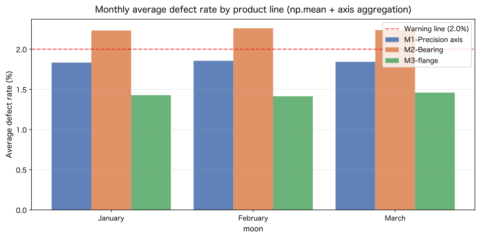

Reading the results

axis=1 calculates the average of each row (line) of the (3, 90) array, We were able to obtain the average defect rate for three lines in one line.
You can compare monthly defect rate changes across the line from the bar graph.
M2-Bearing has remained close to the warning line (2.0%) for the entire month. It can be identified as a priority line for improvement.
You can visually check whether the monthly trend is improving or worsening.

---

No.068: Calculate maximum and minimum values

Practical meaning

“When was the day when the defect rate was the highest?” “Which line was the day when the number of production was the lowest?” To answer this question, you need both the maximum and minimum values and their index (what day).
np.argmax() / np.argmin() allows you to identify values ​​and dates at the same time.

Concept of analysis and modeling

np.max() returns the maximum value, but “which position” is obtained using np.argmax().
To convert from daily index (0-based) to actual date: Use base_date + datetime.timedelta(days=idx).
It can be used to automate the process of regularly identifying and reporting the “worst day” within a month.

Check with Python

import datetime

# Maximum/minimum defect rate for the entire period
overall_max = float(np.max(defect_rates_2d))
overall_min = float(np.min(defect_rates_2d))

print(f"=== Extreme value of defect rate for all lines and all periods ===")
print(f"  Maximum defect rate : {overall_max:.2f}%")
print(f"  Minimum defect rate : {overall_min:.2f}%")
print()

# Identify the worst and best days for each line
print(f"{'line':<14} {'Maximum defect rate':>10} {'worst day':>10} {'Minimum defect rate':>10} {'best day':>10}")
print("=" * 56)
for i, line in enumerate(lines):
    max_dr   = float(defect_rates_2d[i].max())
    min_dr   = float(defect_rates_2d[i].min())
    max_day  = int(np.argmax(defect_rates_2d[i]))
    min_day  = int(np.argmin(defect_rates_2d[i]))
    max_date = (base_date + datetime.timedelta(days=max_day)).strftime("%m/%d")
    min_date = (base_date + datetime.timedelta(days=min_day)).strftime("%m/%d")
    print(f"  {line:<14} {max_dr:>9.2f}% {max_date:>10} {min_dr:>9.2f}% {min_date:>10}")

print()
# Day with the highest production total for all lines
daily_total_prod = prod_2d.sum(axis=0)    # shape: (90,)
best_day_idx     = int(np.argmax(daily_total_prod))
worst_day_idx    = int(np.argmin(daily_total_prod))
best_date  = (base_date + datetime.timedelta(days=best_day_idx)).strftime("%m/%d")
worst_date = (base_date + datetime.timedelta(days=worst_day_idx)).strftime("%m/%d")
print(f"=== Total of all lines Extreme value of production number ===")
print(f"  maximum production date: {best_date}  ({int(daily_total_prod[best_day_idx]):,} units)")
print(f"  Minimum production date: {worst_date}  ({int(daily_total_prod[worst_day_idx]):,} units)")

=== Extreme value of defect rate for all lines and all periods === Maximum defect rate: 2.89% Minimum defect rate: 0.90%

Line Maximum defect rate Worst day Minimum defect rate Best day
=========================================================
  M1-Precision axis 2.55% 01/15 1.32% 03/20
  M2-Bearing 2.89% 01/18 1.53% 01/11
  M3-Flange 1.94% 01/15 0.90% 03/20

=== Total of all lines Extreme value of production quantity ===
  Maximum production date: 03/02 (1,433 pieces)
  Minimum production date: 03/24 (1,322 pieces)

Reading the results

np.argmax(defect_rates_2d[i]) takes the index of the “worst day” of each line, I converted it to an actual date with base_date + timedelta(days=idx).
If the worst day (maximum defect rate day) differs from line to line, root cause analysis must be performed separately.
If the defect rate of multiple lines is high on the same day, check the common factors** (material lots, workers, environment). It is efficient to prioritize research.

---

No.069: Calculate standard deviation

Practical meaning

Even if the average defect rate is the same, lines with large dispersion (standard deviation) are The quality is not stable from day to day, making it difficult to manage.
Using the coefficient of variation (CV = standard deviation / mean), You can horizontally compare the stability of lines with different units and levels.

Concept of analysis and modeling

np.std(data) returns the population standard deviation (denominator = n).
For sample estimation, use np.std(data, ddof=1) (sample standard deviation, denominator = n-1).
At manufacturing sites, population standard deviation is often used as “all production days of this month = population”.
Standard deviation is the basic metric when calculating Process Capability Index (Cp/Cpk), such as dimension measurements.

Check with Python

# Evaluate quality stability with np.std(), np.var()

print(f"{'line':<14} {'Average defect rate':>10} {'standard deviation':>10} {'Coefficient of variation CV':>12} {'Stability evaluation':>12}")
print("=" * 62)
for i, line in enumerate(lines):
    mean_v = float(np.mean(defect_rates_2d[i]))
    std_v  = float(np.std(defect_rates_2d[i]))       # population standard deviation
    cv_pct = std_v / mean_v * 100
    stability = "◎ Stable" if cv_pct < 10 else ("○ Normal" if cv_pct < 20 else "△ Unstable")
    print(f"  {line:<14} {mean_v:>9.2f}% {std_v:>9.3f}% {cv_pct:>10.1f}% {stability:>12}")

print()

# Dimensional inspection: Calculation of process capability index (Cp)
print("=== M1-Precision shaft shaft diameter process capability evaluation ===")
mu_m    = float(np.mean(measurements))
sigma_m = float(np.std(measurements))    # population standard deviation
usl     = target_diam + tolerance        # Upper limit specification value
lsl     = target_diam - tolerance        # Lower limit specification value
cp      = (usl - lsl) / (6 * sigma_m)   # Process capability index Cp
cpk     = min(usl - mu_m, mu_m - lsl) / (3 * sigma_m)   # Cpk (bias consideration)

print(f"  Target value: {target_diam:.3f} mm  Tolerance: ±{tolerance:.3f} mm")
print(f"  Measurement average: {mu_m:.4f} mm  standard deviation: {sigma_m:.4f} mm")
print(f"  Cp  = {cp:.2f}  (1.33 Pass with above: {'✅ Passed' if cp >= 1.33 else '❌ Needs improvement'})")
print(f"  Cpk = {cpk:.2f}  (1.33 Pass with above: {'✅ Passed' if cpk >= 1.33 else '❌ Needs improvement'})")
print()
n_ng = int(np.sum((measurements < lsl) | (measurements > usl)))
print(f"  Out of tolerance product: {n_ng} units / {len(measurements)} units")

Line Average defect rate Standard deviation Coefficient of variation CV Stability evaluation ============================================================== M1-Precision shaft 1.84% 0.268% 14.6% ○ Normal M2-bearing 2.24% 0.319% 14.2% ○ Normal M3-flange 1.43% 0.217% 15.1% ○ Normal

=== M1-Precision shaft shaft diameter process capability evaluation ===
  Target value: 25.000 mm Tolerance: ±0.050 mm
  Measurement average: 24.9983 mm Standard deviation: 0.0165 mm
  Cp = 1.01 (1.33 or higher: ❌ Needs improvement)
  Cpk = 0.98 (1.33 or higher: ❌ Needs improvement)

  Out of tolerance items: 0 pieces / 30 pieces

Reading the results

Looking at the coefficient of variation (CV), the M3-flange has a high CV; It can be seen that although the average defect rate is low, it is an “unstable line” with large day-to-day variations.
The process capability index Cp is calculated as “standard width / (6σ)”.
When Cp ≥ 1.33 (sufficient process capability), the theoretical defect rate is less than 66ppm (0.0066%).
Cpk is an index that takes into account the center deviation of the process, and if Cp > Cpk, It means that “the variation is small, but the average deviates from the target.”

---

No.070: Extract data that meets the conditions

Practical meaning

The process of “automatically extracting and reporting the days when the defect rate exceeds the warning line (2.0%)” is as follows: It is one of the most frequently required operations in manufacturing data pipelines.
Using NumPy’s Boolean index and np.where(), Conditional filtering can be performed quickly using vector operations.

Concept of analysis and modeling

array[array > threshold] is filtering by boolean index, Returns only the elements that meet the condition as a new array (copy).
np.where(condition, true value, false value) selects two values depending on conditions Array version of the ternary operator. It can be used to automatically add warning labels to management graphs.

Check with Python

# Extracting warning date with boolean index and np.where()
threshold = 2.0  # Warning line (defect rate 2.0%)

print("=== Warning date extraction by Boolean index ===")
for i, line in enumerate(lines):
    alert_mask  = defect_rates_2d[i] > threshold    # boolean array, shape: (90,)
    alert_count = int(alert_mask.sum())
    if alert_count > 0:
        alert_dr = defect_rates_2d[i][alert_mask]   # fancy index
        print(f"  {line}: warning day {alert_count:2d}days / {n_days}days  "
              f"maximum {float(alert_dr.max()):.2f}%  Warning day average {float(alert_dr.mean()):.2f}%")
    else:
        print(f"  {line}: warning day  0days / {n_days}days  (normal all day)")

print()

# Add a label with np.where() (M1 first 10 days)
labels_m1 = np.where(defect_rates_2d[0] > threshold, "🔴 Warning", "✅ Normal")
print("=== Status label by np.where() (M1, first 10 days) ===")
for j in range(10):
    d = (base_date + datetime.timedelta(days=j)).strftime("%m/%d")
    print(f"  {d}: {defect_rates_2d[0, j]:.2f}%  {labels_m1[j]}")

print()
# Day when multiple lines issued a warning at the same time
simultaneous = int(np.sum(np.sum(defect_rates_2d > threshold, axis=0) >= 2))
print(f"2Number of days where above the line was warned on the same day: {simultaneous} days")

=== Warning date extraction by Boolean index === M1-Precision axis: Warning days 26 days / 90 days Maximum 2.55% Warning day average 2.17% M2-Bearing: Warning days 71 days / 90 days Maximum 2.89% Warning day average 2.36% M3-Flange: Warning date 0 days / 90 days (normal all days)

=== Status label by np.where() (M1, first 10 days) ===
  01/01: 1.71% ✅ Normal
  01/02: 1.53% ✅ Normal
  01/03: 2.03% 🔴 Warning
  01/04: 2.06% 🔴 Warning
  01/05: 2.00% ✅ Normal
  01/06: 2.14% 🔴 Warning
  01/07: 1.56% ✅ Normal
  01/08: 1.77% ✅ Normal
  01/09: 1.36% ✅ Normal
  01/10: 1.59% ✅ Normal

Number of days when two or more lines issued a warning on the same day: 21 days

# Daily defect rate trends for all lines + warning day highlights (3 panels)
fig, axes = plt.subplots(3, 1, figsize=(12, 8), sharex=True)
colors_070 = ["#4C72B0", "#DD8452", "#55A868"]
day_range  = np.arange(n_days)

for i, (ax, line) in enumerate(zip(axes, lines)):
    dr         = defect_rates_2d[i]
    alert_mask = dr > threshold

    ax.plot(day_range, dr, color=colors_070[i], linewidth=1.5, alpha=0.7)
    ax.scatter(day_range[alert_mask], dr[alert_mask],
               color="red", zorder=5, s=45, label=f"Warning date ({int(alert_mask.sum())}day)")
    ax.axhline(threshold, color="red", linestyle="--", linewidth=1.0, alpha=0.6)
    ax.set_title(f"{line}  ─  warning day: {int(alert_mask.sum())} days / {n_days} days", fontsize=11)
    ax.set_ylabel("Defect rate (%)", fontsize=10)
    ax.legend(fontsize=9)
    ax.grid(alpha=0.3)

axes[-1].set_xlabel("Daily index (0 = 2024-01-01)", fontsize=11)
plt.suptitle("Daily defect rate trends and warning date extraction by product line (np.where / Boolean index)",
             fontsize=13, y=1.01)
plt.tight_layout()
plt.show()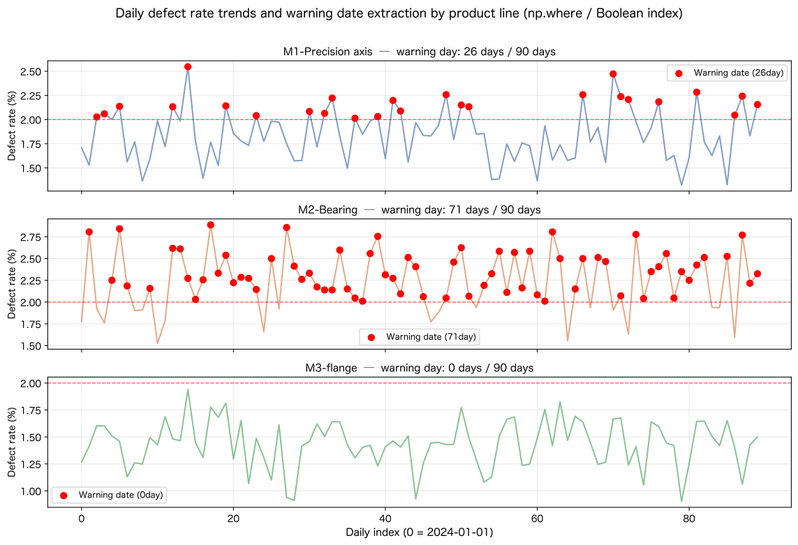

Reading the results

The red dot is the warning date for “defect rate > 2.0%”.
Boolean index of defect_rates_2d[i][alert_mask], We extracted only the data on days that met the conditions and calculated the maximum and average values.
You can visually check the pattern of warning days on the graph.
Defect rate increases before the weekend,'' occurs in clusters at certain times,” etc. If a pattern is visible, identify the cause (equipment maintenance, material lot, worker). This will give you clues to follow.

---

Practical implications seen through target exerciseing

The basics of NumPy learned in No.061-070 are the foundation for speeding up and improving accuracy of manufacturing data analysis.

1. Vector operations = “Code simplicity” and “Scalability”

for Not only does the defect rate calculation written in the loop become one line, Even if the number of lines increases from 3 to 30, the (30, 90) array operates with the same code as (3, 90).
You can write code that is strong enough to scale up manufacturing data.

2. Specifying axis = “Control of aggregation granularity”

By using axis=0 (daily aggregation) and axis=1 (line by line aggregation), You can control “which dimension to leave” by yourself.
Multidimensional aggregation such as “by month, by line, by shift” This is achieved by combining NumPy’s axis and pandas’ groupby.

3. Boolean index = “dynamic filter”

By making warning lines, control limits, and tolerance thresholds variables, One line of defect_rates_2d[defect_rates_2d > threshold] You can immediately respond to “re-aggregation due to threshold change”.
Parameterizing thresholds is a highly maintainable quality control system design.

4. Automatic calculation of process capability index (Cp / Cpk)

The process to automatically calculate Cp / Cpk from np.std and tolerance design values is as follows: Directly linked to automatic generation of periodic quality reports.
In Chapter 9 (Data processing using Polars), data from multiple processes is Build a system for batch processing.

What you need to implement in practice

These are the steps to implement NumPy, which you learned in this chapter, into a manufacturing data analysis system.

Step 1: NumPy array conversion of CSV data (about half a day)

Load existing Excel/CSV data with np.loadtxt() or np.genfromtxt().
If there are missing values, use np.genfromtxt(file, filling_values=np.nan).

Step 2: Designing a 2D array (about 1 day)

First decide which axis is the line and which axis is the date, Manage all data in the unified format of (n_lines, n_days).
By unifying the shaft design, mistakes in axis specification can be prevented.

Step 3: Creating a file of threshold parameters (about half a day)

Design the system to read threshold values such as warning lines, control limits, and tolerances from CSV or JSON files.
You can now recalculate just by changing the threshold without modifying the code.

Step 4: Automatic reporting of process capability index (about 1 day)

Apply Cp / Cpk calculation in this chapter No.069 to all lines, Build a script to automatically generate monthly quality reports.
In Chapter 10 (Aggregation, Visualization, and Mini-Analysis), we will develop this into a more full-fledged report.

Summary

We will summarize what we learned in this chapter (No.061-070).

No.	Skills	Utilization at manufacturing sites
061	Understanding the role of NumPy	Comparing speed and readability with Python lists, and experiencing vector operations
062	Import NumPy	List of main functions and understand their uses in manufacturing data analysis
063	Create a NumPy array	Array the production number, defective number, and dimension measurements
064	Check the array shape	Understand the two-dimensional structure with shape/ndim/dtype/size
065	Retrieving elements from an array	Understanding indexes, slices, and view vs copy
066	Batch calculation for array	Calculate 270 KPIs in one line using broadcast
067	Calculate the average	axis Batch calculation of line and monthly averages and bar graph visualization
068	Calculating maximum and minimum values	Identifying the worst and best days using argmax/argmin
069	Calculate standard deviation	Evaluate stability using coefficient of variation and calculate process capability index using Cp/Cpk
070	Extract data that meets conditions	Automatically extract warning dates with Boolean index and visualize with scatter plot

Chapter 8 (No.071-080) uses Polars, Treat the NumPy array in this chapter as a DataFrame, Learn aggregation, filtering, and CSV loading using column names.

Consultation for corporations

---

Surikobo provides Python training and data analysis support for manufacturing industry and DX promotion staff.

Do you have any of these problems?

• “I want to use my company’s actual data to calculate the defect rate and process capacity in this chapter.”
• “I want to automate my quality control system with NumPy”
• “I want to create an automatic calculation tool for control charts (Xbar-R control charts) and process capability index”
• “I would like you to customize your in-house Python training and implement it for the manufacturing industry.”

Services provided

Service	Overview
Python training for the manufacturing industry	Practical training using field data (online/face-to-face)
Quality control automation system	Automatic calculation and reporting of defect rate, Cp/Cpk, and control chart
Sensor data analysis platform	Anomaly detection and predictive maintenance system construction for time-series data
DX promotion consulting	Consistent support from problem resolution to implementation and establishment support

---

📩 Contact: surikobo.co.jp/contact Please feel free to contact us first.