Make manufacturing KPIs reusable with functions, modules, and exception handling

100 Exercises Chapter 5 (No.041-No.050): Functions/Modules/Exception Handling

This article is Chapter 5 of the “100 Exercises on Introduction to Python for Data Analysis” series.
In Chapter 4 (No.031-040), we learned conditional branching and repetition processing.
This chapter covers reusing code with functions, utilizing standard libraries (math, datetime), Robust data pipeline with try-except, Learn KPI calculations for harness production lines.

[!NOTE] This material is a notebook that has been used in corporate training by Surikobo (or its representative, Hiroshi Wayama) in the past, and has been reorganized and edited with the permission of the company and published.
All published data is fictitious and has no relation to actual companies, factories, or numbers.

Introduction: Practical issues in the manufacturing industry covered in this article

This is weekend work for Mr. T, the quality control team at the harness manufacturing factory.

Repeated work every weekend
  1. Manually calculate daily production volume, defect rate, and utilization rate for each of the five product lines.
  2. Copied and revised the defect rate calculation formula for 5 lines x 5 days, a total of 25 times.
  3. Calculate the estimated delivery date using Notepad by adding the lead time days to the parts order date.
  4. Processing stops due to "Unable to convert string to number" error when loading CSV

If you master Python’s functions, standard library, and exception handling, 25 copies into one function call, calendar calculation into one line of code, You can turn a pipeline that stops due to an error into a robust processing flow.

Common situations in the field

Scene	Task
Repeat KPI calculations	Manually calculate defect rate and operating rate by copying and pasting 5 lines
Calculating order quantity	Use a calculator to calculate the required integer order quantity from minimum stock, lead time, and daily consumption amount
Confirm delivery date	Perform calendar calculation of order date + lead time days using Notepad
CSV error handling	If a string is mixed in a numeric field, the entire process will stop
Identifying the cause of the error	It takes time to resolve the problem because you don’t know what happened in which row or column

In the situation where you write the same code for 5 lines, Sign of functionalization. In this chapter, you will learn the solution.

Why is this problem difficult to judge?

Functions, modules, and exception handling have the following pitfalls.

1. Forgot to write return Without return, the function return value will be None.
   Even if result = calc_revenue(...), result cannot be aggregated as None

2. Function scope misunderstanding Variables defined within a function are not visible outside the function.
   As a general rule, avoid overusing the global variable and return the required value with return

3. datetime module name conflict After import datetime you need to write datetime.date(...).
   It is easy to get confused when mixed with from datetime import datetime

4. Abuse of except Exception Catching all errors in one hides unexpected bugs.
   Specify specific types such as ZeroDivisionError, ValueError, KeyError

Overall picture of the exercises covered in this chapter

No.	Title	Usage in manufacturing industry
041	Define a function	Create a common function for defect rate calculation/Batch calculation for 5 lines
042	Using arguments	KPI format function with default argument *args
043	Using the return value	Simultaneously return defect rate, non-defect rate, and cycle time using a tuple
044	Create a function to calculate sales amount	Batch calculation and visualization of 5 lines of non-defective product sales, defective loss, and net profit
045	Create a function to calculate the average value	Average, standard deviation, coefficient of variation of daily defect rate and weekly trend graph
046	Importing the standard library	Importing and basic confirmation of math, datetime, and statistics
047	Using the math module	Rounding up the order quantity and calculating the 95% confidence interval for the defect rate
048	Using the datetime module	Calculating order date → scheduled delivery date, shift working hours, and number of days remaining at the end of the month
049	Handling errors with try-except	Safely handling type errors, missing columns, and value abnormalities when reading CSV
050	Sorting out errors that tend to occur in data processing	Systematically organizing five types of error patterns and countermeasures

Preparing the Python environment

import subprocess, sys

res = subprocess.run(["sw_vers", "-productVersion"], capture_output=True, text=True)
print(f"macOS : {res.stdout.strip()}")
print(f"Python: {sys.version}")

macOS : 26.3
Python: 3.13.1 (main, Dec  3 2024, 17:59:52) [Clang 16.0.0 (clang-1600.0.26.4)]

import numpy as np
import matplotlib
import matplotlib.pyplot as plt
import matplotlib.ticker as ticker

matplotlib.rcParams['font.family'] = 'Hiragino Maru Gothic Pro'
%config InlineBackend.figure_format = 'svg'
np.random.seed(42)

print("Library loading completed")
print(f"  NumPy     : {np.__version__}")
print(f"  Matplotlib: {matplotlib.__version__}")

Library loading completed NumPy: 2.5.1 Matplotlib: 3.11.0

Creation of fictitious data

Assumed scenario: Auto parts factory/harness production line quality control team Period: 3rd week of January 2024 (Monday to Friday, 5 days operation) Management target: 5 product lines (different product names, unit prices, and standard defect rates)

# Daily production data for 5 product lines x 5 days (2024-01-15~19)
lines = ["HA-01", "HA-02", "HB-01", "HB-02", "HC-01"]
line_names = ["harness A-thin", "Harness A-Medium", "harness B-thin", "Harness B-Medium", "harness C-thin"]
unit_prices = [1200, 1350, 980, 1100, 850]  # yen/piece

day_labels = ["Month (1/15)", "Tuesday (1/16)", "Wednesday (1/17)", "Thursday (1/18)", "Fri(1/19)"]

# Daily production number (seed=42)
base_prod = [450, 380, 520, 410, 480]
prod_data = np.array([[int(b + np.random.randint(-15, 16)) for _ in range(5)] for b in base_prod])

# Daily number of defects (standard defect rate 1.2-2.5% + random noise)
dr_base = [0.020, 0.015, 0.025, 0.018, 0.012]
defect_data = np.array(
    [[max(1, int(round(prod_data[i][j] * dr_base[i] + np.random.randn() * 0.8))) for j in range(5)] for i in range(5)]
)

# List of production numbers
print(f"{'line':<8} {'Product name':<16} {'unit price':>8}  {'moon':>4} {'fire':>4} {'water':>4} {'tree':>4} {'money':>4}  {'weekly total':>6}")
print("=" * 65)
for i in range(len(lines)):
    row_str = "  ".join(f"{int(prod_data[i][j]):>4}" for j in range(5))
    print(f"{lines[i]:<8} {line_names[i]:<16} {unit_prices[i]:>8,}  {row_str}  {int(prod_data[i].sum()):>6,}")
print()
print(f"{'line':<8} {'':16} {'Number of defects':>8}  {'moon':>4} {'fire':>4} {'water':>4} {'tree':>4} {'money':>4}  {'weekly total':>6}")
print("=" * 65)
for i in range(len(lines)):
    row_str = "  ".join(f"{int(defect_data[i][j]):>4}" for j in range(5))
    print(f"{lines[i]:<8} {line_names[i]:<16} {'':>8}  {row_str}  {int(defect_data[i].sum()):>6}")

Line Product name Unit price Mon. Tue. Wed. Thu. Fri Weekly total ================================================================== HA-01 Harness A-thin 1,200 441 454 463 449 445 2,252 HA-02 Harness A-Medium 1,350 372 393 385 371 390 1,911 HB-01 Harness B-thin 980 523 527 515 515 528 2,608 HB-02 Harness B-medium 1,100 415 398 402 418 397 2,030 HC-01 Harness C-thin 850 486 485 466 488 476 2,401

Number of defective lines Monday Tuesday Wednesday Thursday Friday Weekly total
==================================================================
HA-01 Harness A-Thin 9 9 9 9 9 45
HA-02 Harness A-Medium 5 6 6 6 6 29
HB-01 Harness B-thin 13 15 11 14 14 67
HB-02 Harness B-Medium 7 8 8 7 6 36
HC-01 Harness C-thin 6 5 4 6 5 26

---

No.041: Define a function

Practical meaning

When copying 5 lines of defect rate calculation formula defects / production * 100, When modifying the calculation logic, you need to modify all 5 locations.
By organizing it into a function (def), you can manage your logic in one place.

Concept of analysis and modeling

Functions are a way to practice the DRY principle (Don’t Repeat Yourself).
Manufacturing KPI calculations include defect rate, utilization rate, cycle time, etc. By defining it as a common function, it can be used even if the number of lines or aggregation period changes. Code changes are kept to a minimum.

Check with Python

# Define a function to calculate defect rate
def defect_rate(defects, production):
    """Returns defect rate (%)"""
    return defects / production * 100


# Single operation check
print("=== Check function operation ===")
print(f"defect_rate(9, 450)  = {defect_rate(9, 450):.2f}%")
print(f"defect_rate(6, 381)  = {defect_rate(6, 381):.2f}%")
print()

# 5 line batch calculation (effect of functionalization)
print(f"{'line':<8} {'weekly production':>8} {'Weekly defective':>8} {'Defect rate':>8}")
print("-" * 38)
for i in range(len(lines)):
    weekly_prod = int(prod_data[i].sum())
    weekly_defects = int(defect_data[i].sum())
    rate = defect_rate(weekly_defects, weekly_prod)
    print(f"{lines[i]:<8} {weekly_prod:>8,} {weekly_defects:>8} {rate:>7.2f}%")

=== Check function operation === defect_rate(9, 450) = 2.00% defect_rate(6, 381) = 1.57%

Line Weekly production Weekly defective defect rate
--------------------------------------
HA-01 2,252 45 2.00%
HA-02 1,911 29 1.52%
HB-01 2,608 67 2.57%
HB-02 2,030 36 1.77%
HC-01 2,401 26 1.08%

Reading the results

By defining one defect_rate(), calculations for 5 lines were completed with the same function call.
Even if the number of lines increases, it can be handled by simply adding one line to the for loop.
This “define once and call as many times as you like” is the biggest advantage of converting into a function.
If you need to change the defect rate calculation formula from * 100 to * 10000, Just modify one line of def defect_rate(...) and it will be reflected on all lines.

---

No.042: Use arguments

Practical meaning

Arguments are values that can be changed depending on the situation, such as “production quantity, defective quantity, unit, accuracy”, etc.
If you use the default argument, you can say “Usually this setting, change only when necessary.” You can create flexible functions. It can be used to generate reports for manufacturing KPIs.

Concept of analysis and modeling

There are four types of arguments: “positional arguments,” “keyword arguments,” “default arguments,” and “variable length arguments (*args).”
In the manufacturing KPI function, if you set “unit, precision, label” as default arguments, While standard reports can be called in one line, special reports can also be supported.

Check with Python

# KPI formatting functions that use default arguments/keyword arguments
def format_kpi(label, value, unit="", precision=2, width=10):
    """Format and return KPI labels and values"""
    formatted = f"{value:.{precision}f}"
    return f"{label}: {formatted:>{width}}{unit}"


# Checking the operation of default arguments
print(format_kpi("Defect rate", 2.02, unit="%"))  # default precision
print(format_kpi("weekly production", 2255, unit="units", precision=0))
print(format_kpi("Operating hours", 7.5, unit="h"))
print()


# Variable length argument with *args: Identify the worst line from the defect rate of multiple lines
def worst_line_idx(*defect_rates):
    """Returns the index and value of the line with the highest defect rate"""
    max_rate = max(defect_rates)
    idx = list(defect_rates).index(max_rate)
    return idx, max_rate


weekly_rates = [defect_rate(int(defect_data[i].sum()), int(prod_data[i].sum())) for i in range(len(lines))]
worst_idx, worst_rate = worst_line_idx(*weekly_rates)
print(f"Highest defect rate line: {lines[worst_idx]}({worst_rate:.2f}%)")
print()


# **kwargs for future expansion
def kpi_header(**metadata):
    """Generate report header"""
    parts = [f"{k}={v}" for k, v in metadata.items()]
    return "[ " + " / ".join(parts) + " ]"


header = kpi_header(factory="Harness manufacturing building", week="2024-W03", shift="Daytime shift")
print(header)

Defect rate: 2.02% Weekly production: 2255 pieces Working time: 7.50h

Highest defect rate line: HB-01 (2.57%)

[factory=Harness manufacturing building / week=2024-W03 / shift=daytime]

Reading the results

format_kpi("Defect rate", 2.02, unit="%") is precision=2 (default) “Defect rate: 2.02%” was output.
Using *args, like worst_line_idx(*weekly_rates) You can pass five numbers as separate arguments.
This allows you to identify the worst line without changing the code even if the number of lines changes.
**kwargs is useful when the number of items is indeterminate, such as report metadata.

---

No.043: Use return value

Practical meaning

There are many situations in manufacturing sites where you want to return multiple KPIs such as “defect rate, good product rate, and cycle time” at the same time in a single calculation.
Python functions can return multiple values in a tuple, so a single call can return You can obtain multiple indicators at once.

Concept of analysis and modeling

If you return the return value as a tuple, you can use “unpacking assignment (a, b, c = func())”, Storing it in a variable can be done in one line.
Select whether to return multiple related indicators as a tuple or as a dictionary ({}).
If you return it as a dictionary, you can use result["defect_rate"] when “only a part of the result is used”. Dictionaries are recommended when there are many output items because they can be retrieved by key.

Check with Python

# A function that returns weekly key KPIs in a dictionary
def production_kpi(production_list, defect_list, unit_price, operated_hours_total):
    """Calculate weekly key KPIs and return them in a dictionary

    Parameters
    ----------
    production_list : list[int] - Daily production number
    defect_list : list[int] - Daily number of defects
    unit_price : int - Unit price (yen/piece)
    operated_hours_total : float - Weekly operating hours (hours)

    Returns
    -------
    dict: total_prod, total_defects, good_units, defect_rate_pct,
          yield_rate_pct, cycle_time_sec, revenue"""
    total_prod = sum(production_list)
    total_defects = sum(defect_list)
    good_units = total_prod - total_defects
    dr_pct = total_defects / total_prod * 100
    yield_pct = good_units / total_prod * 100
    cycle_sec = operated_hours_total * 3600 / total_prod
    revenue = good_units * unit_price
    return {
        "total_prod": total_prod,
        "total_defects": total_defects,
        "good_units": good_units,
        "defect_rate": dr_pct,
        "yield_rate": yield_pct,
        "cycle_time_s": cycle_sec,
        "revenue": revenue,
    }


# Calculate weekly KPIs for HA-01
operated_week = 7.5 * 5  # 7.5h x 5 days
kpi_ha01 = production_kpi(
    production_list=[int(x) for x in prod_data[0]],
    defect_list=[int(x) for x in defect_data[0]],
    unit_price=unit_prices[0],
    operated_hours_total=operated_week,
)

print("=== HA-01 Weekly KPI ===")
print(f"  Total production number     : {kpi_ha01['total_prod']:,} units")
print(f"  Total number of defects     : {kpi_ha01['total_defects']} units")
print(f"  Number of good products       : {kpi_ha01['good_units']:,} units")
print(f"  Defect rate       : {kpi_ha01['defect_rate']:.2f}%")
print(f"  Good product rate (yield): {kpi_ha01['yield_rate']:.2f}%")
print(f"  cycle time: {kpi_ha01['cycle_time_s']:.1f} seconds/units")
print(f"  Good product sales     : {kpi_ha01['revenue']:,.0f} JPY")

=== HA-01 Weekly KPI === Total production: 2,252 pieces Total number of defects: 45 pieces Number of good products: 2,207 pieces Defect rate: 2.00% Good product rate (yield): 98.00% Cycle time: 59.9 seconds/pcs Good product sales: 2,648,400 yen

Reading the results

Since the return value is returned as a dictionary, you can retrieve just any KPI like kpi_ha01["defect_rate"].
Cycle time (cycle_time_s) is automatically calculated from weekly operating hours and total production.
For example, the number {kpi_ha01['cycle_time_s']:.1f} seconds/piece is This is an important indicator for checking the deviation from takt time (planned value).
The same analysis can be applied to all lines such as HB-01 and HC-01 by simply changing the data passed to the function.

---

No.044: Create a function to calculate sales amount

Practical meaning

The formula “Sales of non-defective products - Losses from defects = Net profit” is common to all lines.
The disposal cost rate (penalty_rate) for defective products varies depending on the line, but By setting it as a default argument, normal lines can be processed with the same expression.

Concept of analysis and modeling

We use the following cost calculation model: “Defect loss = number of defects × unit price × (1 + scrapping cost rate)”.
The disposal cost rate is a coefficient that includes “disposal processing cost and re-inspection cost” in addition to “material cost loss”.
penalty_rate=0.3 (30% additional unit price) is a common baseline in manufacturing.

Check with Python

# Functions to calculate sales of non-defective products, loss of non-conforming products, and net profit
def calc_revenue(production, defects, unit_price, penalty_rate=0.30):
    """Calculate weekly revenue metrics

    Parameters
    ----------
    production: int - number of production
    defects : int - number of defects
    unit_price : int - Unit price (yen/piece)
    penalty_rate : float - Defective product scrapping cost rate (default 0.30)

    Returns
    -------
    dict: good_units, revenue, loss, net_revenue, loss_ratio_pct"""
    good_units = production - defects
    revenue = good_units * unit_price
    loss = defects * unit_price * (1 + penalty_rate)
    net_revenue = revenue - loss
    loss_ratio = loss / (revenue + loss) * 100
    return {
        "good_units": good_units,
        "revenue": revenue,
        "loss": loss,
        "net_revenue": net_revenue,
        "loss_ratio_pct": loss_ratio,
    }


# All 5 lines weekly profit calculation
results_044 = []
print(f"{'line':<8} {'Good product sales':>12} {'defect loss':>10} {'net revenue':>12} {'loss rate':>8}")
print("=" * 56)
for i in range(len(lines)):
    prod_w = int(prod_data[i].sum())
    defect_w = int(defect_data[i].sum())
    r = calc_revenue(prod_w, defect_w, unit_prices[i])
    results_044.append(r)
    print(
        f"{lines[i]:<8} {r['revenue']:>12,.0f} {r['loss']:>10,.0f} "
        f"{r['net_revenue']:>12,.0f} {r['loss_ratio_pct']:>7.1f}%"
    )

total_rev = sum(r["revenue"] for r in results_044)
total_los = sum(r["loss"] for r in results_044)
total_net = sum(r["net_revenue"] for r in results_044)
print("=" * 56)
print(f"{'Total':<8} {total_rev:>12,.0f} {total_los:>10,.0f} {total_net:>12,.0f}")

Line Good product sales Defective loss Net income Loss rate ========================================================= HA-01 2,648,400 70,200 2,578,200 2.6% HA-02 2,540,700 50,895 2,489,805 2.0% HB-01 2,490,180 85,358 2,404,822 3.3% HB-02 2,193,400 51,480 2,141,920 2.3% HC-01 2,018,750 28,730 1,990,020 1.4% ========================================================= Total 11,891,430 286,663 11,604,767

# Bar graph of non-defective product sales, defective losses, and net income by line
fig, ax = plt.subplots(figsize=(10, 5))

revenues = [r["revenue"] for r in results_044]
losses = [r["loss"] for r in results_044]
net_revenues = [r["net_revenue"] for r in results_044]

x = np.arange(len(lines))
width = 0.28

ax.bar(x - width, revenues, width, label="Good product sales", color="#4C72B0", alpha=0.88)
ax.bar(x, losses, width, label="defect loss", color="#DD8452", alpha=0.88)
ax.bar(x + width, net_revenues, width, label="net revenue", color="#55A868", alpha=0.88)

ax.set_title("Weekly non-defective product sales, defective losses, and net revenue by product line (3rd week of January 2024)", fontsize=13, pad=10)
ax.set_xlabel("product line", fontsize=11)
ax.set_ylabel("Amount (10,000 yen)", fontsize=11)
ax.set_xticks(x)
ax.set_xticklabels(lines)
ax.yaxis.set_major_formatter(ticker.FuncFormatter(lambda v, _: f"{v/10000:.0f}million"))
ax.legend(fontsize=10)
ax.grid(axis="y", alpha=0.3)
plt.tight_layout()
plt.show()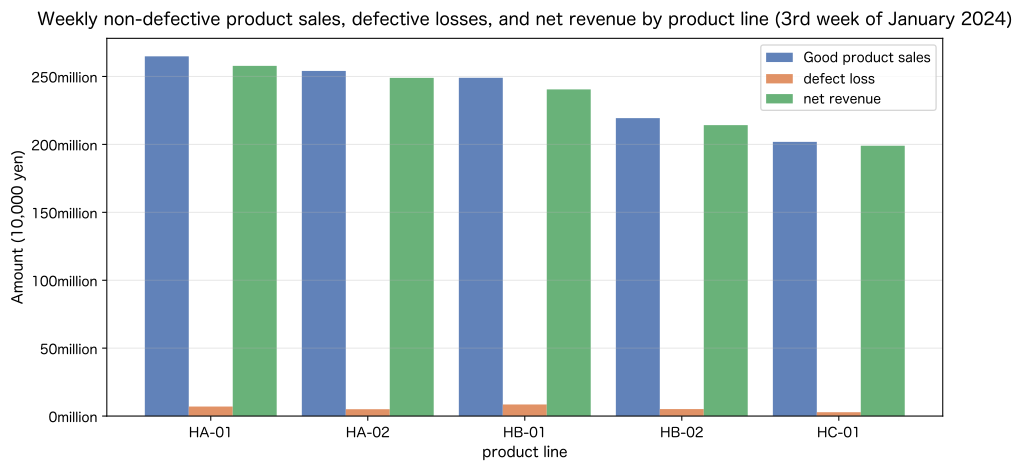

Reading the results

By defining one calc_revenue(), the weekly profits of all 5 lines can be I was able to calculate using the same logic.
From the graph, determine the line with the highest sales of non-defective products and the line with the highest ratio of defective losses. You can compare visually.
Just change penalty_rate=0.30 to penalty_rate=0.50 “Profit simulation after reviewing disposal costs” can be executed immediately.
This is the practice of sensitivity analysis by functionalization.

---

No.045: Create a function to calculate the average value

Practical meaning

By calculating the “average, maximum, minimum, standard deviation, and coefficient of variation” of the daily defect rate of each line, The stability (size of variation) of the manufacturing process can be quantitatively evaluated.
Coefficient of variation (CV = standard deviation / mean) is useful when comparing lines with different units side by side.

Concept of analysis and modeling

Just use sum() and four arithmetic operations without using the Python standard library. By implementing mean, variance, and standard deviation, NumPy’s mean() and std() Understand what’s going on inside.
At manufacturing sites, it is used to determine that a large standard deviation = unstable process.

Check with Python

# Generic function to calculate descriptive statistics (without NumPy)
def calc_stats(data):
    """Calculate the average, maximum, minimum, standard deviation, and coefficient of variation

    Parameters
    ----------
    data : list[float] - numeric list

    Returns
    -------
    dict: mean, max_v, min_v, std, cv_pct"""
    n = len(data)
    mean_v = sum(data) / n
    var = sum((x - mean_v) ** 2 for x in data) / n  # population standard deviation
    std_v = var**0.5
    cv_pct = std_v / mean_v * 100  # Coefficient of variation (%)
    return {
        "mean": mean_v,
        "max_v": max(data),
        "min_v": min(data),
        "std": std_v,
        "cv_pct": cv_pct,
    }


# Calculate the daily defect rate for each line and store it in a list
daily_defect_rates_045 = [[defect_data[i][j] / prod_data[i][j] * 100 for j in range(5)] for i in range(len(lines))]

# Statistics summary table
print(f"{'line':<8} {'Average defect rate':>10} {'maximum':>8} {'minimum':>8} {'standard deviation':>10} {'coefficient of variation':>10}")
print("=" * 60)
for i, line in enumerate(lines):
    s = calc_stats(daily_defect_rates_045[i])
    print(
        f"{line:<8} {s['mean']:>9.2f}% {s['max_v']:>7.2f}% {s['min_v']:>7.2f}%"
        f" {s['std']:>9.3f}% {s['cv_pct']:>9.1f}%"
    )

# Weekly defect rate for all lines total
total_prod_all = int(prod_data.sum())
total_defects_all = int(defect_data.sum())
overall_dr = total_defects_all / total_prod_all * 100
print("=" * 60)
print(f"{'Overall':<8} {overall_dr:>9.2f}%  (total production {total_prod_all:,}units / Total defective {total_defects_all}units)")

Line Average defect rate Maximum Minimum Standard deviation Coefficient of variation ============================================================ HA-01 2.00% 2.04% 1.94% 0.034% 1.7% HA-02 1.52% 1.62% 1.34% 0.092% 6.1% HB-01 2.57% 2.85% 2.14% 0.245% 9.5% HB-02 1.77% 2.01% 1.51% 0.194% 11.0% HC-01 1.08% 1.23% 0.86% 0.140% 13.0% ============================================================ Total 1.81% (Total production 11,202 pieces / Total defective 203 pieces)

# Daily defect rate trend graph (all lines)
fig, ax = plt.subplots(figsize=(10, 5))
colors_045 = ["#4C72B0", "#DD8452", "#55A868", "#C44E52", "#8172B2"]

for i, line in enumerate(lines):
    ax.plot(
        day_labels, daily_defect_rates_045[i], marker="o", label=line, color=colors_045[i], linewidth=2, markersize=6
    )

# Warning line (2.0%)
ax.axhline(2.0, color="red", linewidth=1.5, linestyle="--", alpha=0.7, label="Warning line (2.0%)")

ax.set_title("Daily defect rate trends by product line (3rd week of January 2024)", fontsize=13, pad=10)
ax.set_xlabel("date", fontsize=11)
ax.set_ylabel("Defect rate (%)", fontsize=11)
ax.legend(bbox_to_anchor=(1.02, 1), loc="upper left", fontsize=9)
ax.grid(alpha=0.3)
plt.tight_layout()
plt.show()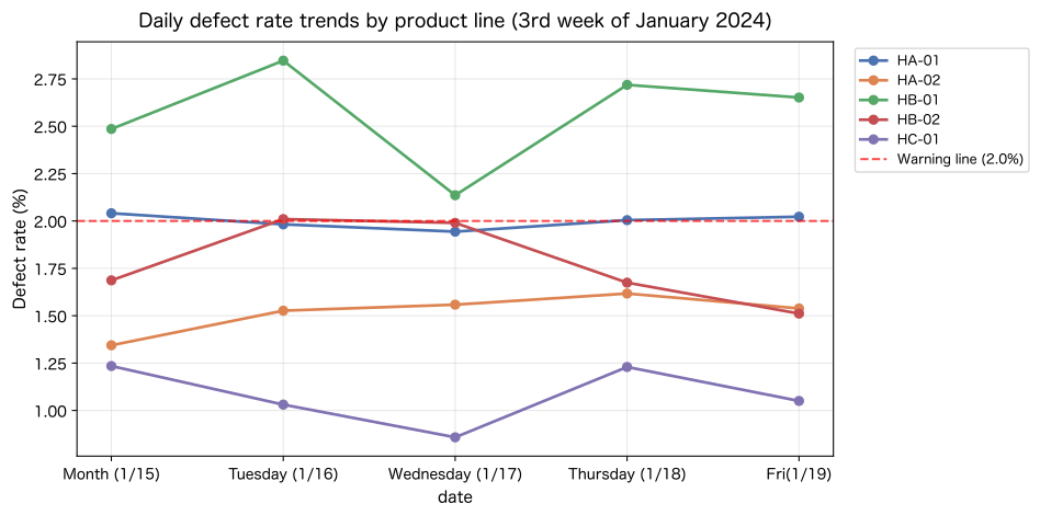

Reading the results

calc_stats() was implemented using only Python built-in functions (sum, max, min) General purpose statistical functions. The standard deviation is calculated using var ** 0.5.
The larger the coefficient of variation (CV), the greater the variation from day to day. Indicates that the process is unstable.
Identify at a glance the date and line that exceeded the warning line (2.0%) on the graph, It can be used for prioritizing factor analysis.

---

No.046: Import standard library

Practical meaning

Python has a rich standard library that can be used without additional installation with pip.
Frequently used in manufacturing data processing are math (mathematics), datetime (date and time), statistics (statistics), csv (CSV read/write) and os (file path).

Concept of analysis and modeling

Load the standard library with import library name.
statistics module can calculate mean, variance, and median without numpy.
However, numpy is required for fast processing of large amounts of data.
Use standard libraries and external libraries depending on the situation.

Check with Python

# Importing standard libraries often used in manufacturing data processing
import math
import datetime
import statistics
import os
import sys

print("=== Standard library confirmation ===")
for name, mod in [("math", math), ("datetime", datetime), ("statistics", statistics), ("os", os), ("sys", sys)]:
    print(f"  {name:<12}: {mod.__name__}")
print()

# Aggregating daily defect rates using the statistics module
all_daily_rates = [defect_data[i][j] / prod_data[i][j] * 100 for i in range(len(lines)) for j in range(5)]

print(f"statistics.mean()    : {statistics.mean(all_daily_rates):.3f}%")
print(f"statistics.median()  : {statistics.median(all_daily_rates):.3f}%")
print(f"statistics.stdev()   : {statistics.stdev(all_daily_rates):.3f}%   # sample standard deviation")
print(f"statistics.variance(): {statistics.variance(all_daily_rates):.4f}")
print()
print(f"  [Reference] No.045 of calc_stats() comparison with")
s = calc_stats(all_daily_rates)
print(f"  calc_stats mean: {s['mean']:.3f}%  / std: {s['std']:.3f}%  (population standard deviation)")

=== Standard library confirmation ===

math: math datetime: datetime statistics: statistics os : os sys: sys

statistics.mean() : 1.788%
statistics.median() : 1.687%
statistics.stdev() : 0.531% # Sample standard deviation
statistics.variance(): 0.2819

  [Reference] Comparison with No.045 calc_stats()
  calc_stats mean: 1.788% / std: 0.520% (population standard deviation)

Reading the results

statistics.stdev() uses sample standard deviation (denominator n-1).
On the other hand, std of No.045 calc_stats() is the population standard deviation (denominator n).
When the sample is small, this difference affects statistical inference.
Manufacturing data can often be considered as “this week’s entire production = population”, so There are also situations where the population standard deviation is used.
The default of numpy’s np.std() is the population standard deviation (ddof=0), so Please keep in mind that there is a difference between statistics.stdev() and statistics.stdev().

---

No.047: Use math module

Practical meaning

A typical example of how to use the math module at a manufacturing site is ① Round up calculation (math.ceil) of order quantity ② Confidence interval calculation (math.sqrt) in statistical quality control.
math.ceil is required for the constraint that “the number of orders cannot be reduced to a small number”.

Concept of analysis and modeling

math.ceil(x) returns the smallest integer greater than x.
When calculating the order quantity, round() may be truncated. There is a risk of falling below the minimum stock. In the manufacturing industry, the general rule is to round to the safe side (more).
The 95% confidence interval ($\hat{p} \pm 1.96\sqrt{\hat{p}(1-\hat{p})/n}$) is This is a basic indicator of statistical quality control (SQC) that indicates the accuracy of estimating defect rate.

Check with Python

import math

# Calculation of order quantity rounding up
min_stock_47 = 200  # Minimum stock quantity (pieces)
current_stock_47 = 143  # Current stock quantity (pieces)
daily_usage_47 = 18.7  # Average daily usage (pcs/day)
lead_days_47 = 5  # Order lead time (days)

# Consumption amount during order period + minimum stock maintenance amount
order_exact = (min_stock_47 - current_stock_47) + daily_usage_47 * lead_days_47
order_qty = math.ceil(order_exact)  # Round up to whole number

print(f"=== Order quantity calculation ===")
print(f"  Shortage in stock       : {min_stock_47 - current_stock_47} units")
print(f"  Lead time consumption  : {daily_usage_47} × {lead_days_47} = {daily_usage_47 * lead_days_47:.1f} units")
print(f"  Theoretical order quantity (There are fractions): {order_exact:.2f} units")
print(f"  Actual number of orders (Kirigami): {order_qty} units  ← math.ceil() Applicable")
print()

# 95% confidence interval for weekly defect rate
total_prod_47 = int(prod_data.sum())
total_defects_47 = int(defect_data.sum())
p_hat = total_defects_47 / total_prod_47
hw = 1.96 * math.sqrt(p_hat * (1 - p_hat) / total_prod_47)

print(f"=== Defect rate 95% confidence interval ===")
print(f"  Total production number  : {total_prod_47:,} units")
print(f"  Total number of defects  : {total_defects_47} units")
print(f"  Defect rate estimate: {p_hat*100:.4f}%")
print(f"  95% CI      : [{(p_hat-hw)*100:.4f}%, {(p_hat+hw)*100:.4f}%]")
print()

# math function reference
print("=== math main functions ===")
print(f"  math.ceil(3.2)    : {math.ceil(3.2)}")
print(f"  math.floor(3.8)   : {math.floor(3.8)}")
print(f"  math.sqrt(2)      : {math.sqrt(2):.6f}")
print(f"  math.log(math.e)  : {math.log(math.e):.6f}  # natural logarithm")
print(f"  math.log10(1000)  : {math.log10(1000):.6f}  # common logarithm")
print(f"  math.pi           : {math.pi:.6f}")

=== Order quantity calculation === Insufficient stock: 57 pieces Lead time consumption: 18.7 × 5 = 93.5 pieces Theoretical order quantity (with fractions): 150.50 pieces Actual number of orders (rounded up): 151 pieces ← math.ceil() applied

=== Defect rate 95% confidence interval ===
  Total production: 11,202 pieces
  Total number of defects: 203 pieces
  Defect rate estimate: 1.8122%
  95% CI: [1.5652%, 2.0592%]

=== math main functions ===
  math.ceil(3.2) : 4
  math.floor(3.8) : 3
  math.sqrt(2) : 1.414214
  math.log(math.e) : 1.000000 # natural logarithm
  math.log10(1000) : 3.000000 # Common logarithm
  math.pi : 3.141593

Reading the results

math.ceil(order_exact) rounded up the theoretical order quantity and calculated the order quantity in whole numbers.
round() and int() are rounded down and there is a risk of inventory shortage. math.ceil is safe for order calculations in the manufacturing industry.
A 95% confidence interval for a defect rate means that there is a 95% chance that this range contains the true defect rate.
The larger the number of products produced, the narrower the CI width (the higher the estimation accuracy). The same concept is used to calculate the defect rate control chart (control limit line).

---

No.048: Use datetime module

Practical meaning

The main uses of datetime at manufacturing sites are ①** Calculation of scheduled delivery date** (order date + number of lead time days) ②** Calculation of shift working time** (end time − start time − break time) ③Check the number of days remaining until the end of the month/period (calculation of remaining amount of production plan) There are three. These can be automated by manual calculation or by visually checking the calendar.

Concept of analysis and modeling

Focusing on two classes: datetime.date and datetime.timedelta You can add and subtract dates.
timedelta(days=5) is a “time difference object” for calculating “5 days later”.
By converting to a format string with strftime(), You can automatically generate date displays for reports and notification emails.

Check with Python

import datetime

# Calculate the estimated delivery date from the order date
order_date_48 = datetime.date(2024, 1, 15)  # Ordered on Monday
lead_days_48 = 5
delivery_date_48 = order_date_48 + datetime.timedelta(days=lead_days_48)

print("=== Order/Delivery Schedule ===")
print(f"  Order date      : {order_date_48.strftime('%Y-%m-%d (%a)')}")
print(f"  lead time: {lead_days_48} days")
print(f"  Expected delivery date  : {delivery_date_48.strftime('%Y-%m-%d (%a)')}")
print()

# Shift working time calculation
shift_start_48 = datetime.datetime(2024, 1, 15, 8, 0, 0)
shift_end_48 = datetime.datetime(2024, 1, 15, 17, 0, 0)
break_time_48 = datetime.timedelta(minutes=60)
worked_td = shift_end_48 - shift_start_48 - break_time_48
worked_hours_48 = worked_td.total_seconds() / 3600

print("=== Shift Working Time ===")
print(f"  Start of shift: {shift_start_48.strftime('%H:%M')}")
print(f"  End of shift: {shift_end_48.strftime('%H:%M')}")
print(f"  Break time  : 60 minutes")
print(f"  Actual operating time: {worked_hours_48:.1f} hours")
print()

# Number of days remaining until the end of the month/weekend
today_48 = datetime.date(2024, 1, 19)  # Friday of the 3rd week
month_end = datetime.date(2024, 1, 31)
remaining_days = (month_end - today_48).days

print("=== Number of days remaining until the end of the month ===")
print(f"  Today  : {today_48}")
print(f"  end of month  : {month_end}")
print(f"  Remaining days: {remaining_days} days")
print()

# Automatically generates 5-day production schedule dates
print("=== Weekly production schedule ===")
weekday_map = {0: "moon", 1: "fire", 2: "water", 3: "tree", 4: "money", 5: "soil", 6: "days"}
for d in range(5):
    dt = order_date_48 + datetime.timedelta(days=d)
    prod_total = int(prod_data[:, d].sum())
    print(f"  {dt.strftime('%m/%d')} ({weekday_map[dt.weekday()]})  Total production of all lines: {prod_total:,} units")

=== Order/Delivery Schedule === Order date: 2024-01-15 (Mon) Lead time: 5 days Scheduled delivery date: 2024-01-20 (Sat)

=== Shift Working Time ===
  Shift start: 08:00
  End of shift: 17:00
  Break time: 60 minutes
  Actual working time: 8.0 hours

=== Number of days remaining until the end of the month ===
  Today: 2024-01-19
  End of month: 2024-01-31
  Remaining days: 12 days

=== Weekly production schedule ===
  01/15 (Monday) Total production of all lines: 2,237 pieces
  01/16 (Tue) Total production of all lines: 2,257 pieces
  01/17 (Wed) Total production of all lines: 2,231 pieces
  01/18 (Thu) Total production for all lines: 2,241 pieces
  01/19 (Fri) Total production for all lines: 2,236 pieces

Reading the results

By using datetime.timedelta(days=5), you can set the estimated delivery date 5 days after the order date. I was able to calculate it in one line. Calendar calculations that span weekends and month-ends are automatically and accurately processed.
total_seconds() / 3600 converts shift working time into hours.
datetime.timedelta can handle days, hours, minutes, seconds, and microseconds, so It can also be applied to time stamp difference calculation of equipment operation logs.

---

No.049: Handle errors with try-except

Practical meaning

Data from sensors and CSV files manually entered by operators are “There are characters in the numeric field,” “There are not enough columns,” “There are negative numbers,” etc. Abnormal data will be mixed in. Without try-except, the entire process will stop the moment an error occurs.
Continue to aggregate only good rows while handling errors is a requirement for manufacturing data pipelines.

Concept of analysis and modeling

If an error occurs in the try block, processing moves to the corresponding except block.
By writing multiple except, you can branch processing depending on the type of error.
finally block is always executed regardless of success or failure, so It is used for file closing processing (details will be covered in Chapter 6).

Check with Python

# Function to safely parse a single line of CSV
def safe_parse_row(row, row_num=0):
    """Parse one CSV line (list format) and return result dictionary or error dictionary

    Expected error
    ----------
    IndexError: Insufficient number of columns
    ValueError: Type conversion failure/value error"""
    try:
        product_code = row[0]  # Part number (string)
        production = int(row[1])  # Production number → int conversion
        defects = int(row[2])  # Number of defects → int conversion
        unit_price = float(row[3])  # Unit price → float conversion

        # Validation of business rules
        if production <= 0:
            raise ValueError(f"Production quantity must be a positive integer: {production}")
        if defects > production:
            raise ValueError(f"Number of defects({defects})is the number of production({production})exceeds")

        dr = defects / production * 100
        return {
            "code": product_code,
            "production": production,
            "defects": defects,
            "unit_price": unit_price,
            "defect_rate": dr,
        }

    except IndexError:
        return {"error": f"rows{row_num}: Insufficient number of columns ({len(row)} column)", "row": row}
    except ValueError as e:
        return {"error": f"rows{row_num}: Value error ({e})", "row": row}


# Test data (normal/abnormal mixture)
test_rows_049 = [
    ["HA-01", "450", "9", "1200"],  # ✅ Normal
    ["HA-02", "381", "6", "1350"],  # ✅ Normal
    ["HB-01", "525", "abc", "980"],  # ❌ ValueError (number of defects is a string)
    ["HB-02", "415"],  # ❌ IndexError (missing columns)
    ["HC-01", "485", "520", "850"],  # ❌ ValueError (Number of defects > Number of production)
    ["HC-01", "0", "0", "850"],  # ❌ ValueError (production quantity = 0)
]

print("=== CSV row analysis result ===")
ok_rows, ng_rows = [], []
for i, row in enumerate(test_rows_049, start=1):
    result = safe_parse_row(row, row_num=i)
    if "error" in result:
        ng_rows.append(result)
        print(f"  ❌ {result['error']}")
    else:
        ok_rows.append(result)
        print(f"  ✅ rows{i}: {result['code']}  production{result['production']:>4}units  " f"Defect rate{result['defect_rate']:.2f}%")

print()
print(f"Normal processing: {len(ok_rows)} rows / skip: {len(ng_rows)} rows")

=== CSV row analysis result === ✅ Row 1: HA-01 Production 450 pieces Defect rate 2.00% ✅ Row 2: HA-02 Production 381 pieces Defect rate 1.57% ❌ Line 3: Value error (invalid literal for int() with base 10: ‘abc’) ❌ Row 4: Insufficient number of columns (2 columns) ❌ Line 5: Value error (number of defects (520) exceeds number of production (485)) ❌ Line 6: Value error (production quantity must be a positive integer: 0)

Successful processing: 2 lines / Skip: 4 lines

Reading the results

safe_parse_row() processed 6 lines of test data and accurately distributed 2 normal lines and 4 error lines.
The row with the error is returned as {"error": ..., "row": ...}, so You can later report a list of errors and request manual correction.
except IndexError and except ValueError are written separately, so You can keep an error log that distinguishes between “missing columns” and “wrong values.”
There are two golden rules for manufacturing data pipelines: “Do not stop due to errors and leave errors in the log.”

---

No.050: Sort out errors that tend to occur in data processing

Practical meaning

There are certain patterns of errors that occur in manufacturing data processing.
5 types of errors (ZeroDivisionError/KeyError/TypeError/ValueError/IndexError) By systematically understanding them and preparing appropriate solutions as codes, This can significantly reduce troubleshooting time in the production environment.

Concept of analysis and modeling

Error handling is the basis of “defensive programming”.
Anticipate in advance what will be included in this data, try-except can be combined with pre-validation (confirmation with if statement). Design principles for robust data pipelines.

Check with Python

# 5 types of errors that frequently occur in data processing and how to deal with them

error_catalog = [
    {
        "type": "ZeroDivisionError",
        "scene": "Defect rate calculation when production quantity is 0",
        "trigger": "defects / production * 100  (production=0)",
        "fix": "Check production > 0 or try-except",
    },
    {
        "type": "KeyError",
        "scene": "Accessing keys not present in dictionary",
        "trigger": "part_info['supplier'] (key not registered)",
        "fix": "part_info.get('supplier', 'unknown')",
    },
    {
        "type": "TypeError",
        "scene": "String and number operations",
        "trigger": "'326' + 15  (str + int)",
        "fix": "Type conversion with int('326') + 15",
    },
    {
        "type": "ValueError",
        "scene": "Convert unconvertable strings to numbers",
        "trigger": "int('12a') (non-numeric string)",
        "fix": "Skip with try-except ValueError",
    },
    {
        "type": "IndexError",
        "scene": "List out-of-bounds access",
        "trigger": "row[5] (CSV with only 5 columns)",
        "fix": "Check len(row) > 5 or try-except",
    },
]

print(f"{'Error type':<22} {'Occurrence scene':<28} {'How to deal with it'}")
print("=" * 80)
for e in error_catalog:
    print(f"{e['type']:<22} {e['scene']:<28} {e['fix']}")
print()

# try-except demonstration of each error
print("=== try-except demonstration ===")

# ZeroDivisionError
try:
    rate_050 = 3 / 0
except ZeroDivisionError:
    rate_050 = None
print(f"ZeroDivisionError → rate = {rate_050}  (None Set and continue processing)")

# KeyError (avoided with get())
part_info_050 = {"code": "HA-01", "production": 450}
supplier_050 = part_info_050.get("supplier", "Not registered")
print(f"KeyError avoidance     → supplier = '{supplier_050}'  (get() default value of)")

# TypeError
try:
    result_050 = "326" + 15
except TypeError:
    result_050 = int("326") + 15
print(f"TypeError avoidance    → result = {result_050}  (int() Convert and recalculate with)")

# ValueError
try:
    v_050 = int("12a")
except ValueError as e:
    v_050 = None
    e_msg_050 = str(e)
print(f"ValueError avoidance   → v = {v_050}  ('{e_msg_050}' → skip)")

# IndexError
row_050 = ["HC-01", "480"]
try:
    defects_050 = int(row_050[2])
except IndexError:
    defects_050 = 0
print(f"IndexError avoidance   → defects = {defects_050}  (Not enough rows → default0set)")

Error type Occurrence situation Remedy ================================================================================ ZeroDivisionError Calculate defect rate with production number 0 Check production > 0 or try-except KeyError Accessing a key that does not exist in the dictionary part_info.get(‘supplier’, ‘unknown’) TypeError String and number operation int(‘326’) + 15 type conversion ValueError Convert unconvertable strings to numbers Skip with try-except ValueError IndexError List out-of-bounds access len(row) > 5 or try-except

=== try-except demonstration ===
ZeroDivisionError → rate = None (Set None and continue processing)
Avoid KeyError → supplier = 'unregistered' (default value of get())
Avoid TypeError → result = 341 (convert with int() and recalculate)
Avoid ValueError → v = None ('invalid literal for int() with base 10: '12a'' → skip)
Avoid IndexError → defects = 0 (missing column → set default to 0)

Reading the results

We have organized a list of 5 types of errors and how to deal with them.
In an actual data pipeline, you can choose to return an error,'' use default value,” or “skip and log.” Choose from three options depending on the situation.

Response policy	When to use
Set None and continue processing	When it can be treated as missing in aggregation processing
Default value (get(), etc.)	If the key or column is an optional item
Skip with except + Log	Excluding abnormal rows and counting only normal rows
Retransmit with raise	In case of serious abnormality that should notify the caller of the error

The design of “which errors to ignore and which errors to notify” It determines the quality of your manufacturing data pipeline.

---

Practical implications seen through target exerciseing

The “functions, modules, and exception handling” learned in No.041-050 are These are the basic skills that determine the design quality of a manufacturing KPI system.

1. Functionalization = “Reduction of maintenance costs”

A code with 5 lines of the same calculations would need to be modified in 5 places every time the specifications change.
By consolidating into one function like calc_revenue(), Changes in specifications can be reflected in the entire line with a single modification.
At manufacturing sites, the number of lines increases/the definition of KPIs changes, so Functionalization is a design that increases resistance to change.

2. Standard library = “No installation required productivity tools”

Rounding up the order quantity using math.ceil Delivery date calculation using datetime.timedelta is Ready to use without any additional libraries.
Even in a manufacturing IT environment where a request to install a tool is not successful. Many tasks can be automated using the standard library.

3. Exception handling = “Data pipeline quality assurance”

Sensor data/manually input CSV will always contain abnormal values.
In a system without try-except, the entire process will stop if one error occurs.
By implementing a function like safe_parse_row(), “We continue to process 99% of normal data without stopping. “Accumulate only abnormal data in the log and check it later.” The ideal operation of the manufacturing data pipeline can be achieved.

What you need to implement in practice

This section describes the steps to implement what you have learned in this chapter into your manufacturing site data system.

Step 1: Creating a KPI function library (about 1 day)

Use the functions created in this chapter such as defect_rate(), calc_revenue(), calc_stats(), etc. Combine them into one file as kpi_functions.py.
Can be reused with from kpi_functions import calc_revenue from other notebook scripts.

Step 2: Schedule automation using datetime (about half a day)

Implement the calculation of order date, scheduled delivery date, and number of days remaining at the end of the month using the datetime function, Automate daily routine tasks (order alerts, schedule confirmation).

Step 3: Build a secure CSV loading pipeline (about 1 day)

Use safe_parse_row() to “summarize only normal rows while skipping abnormal rows” Build the loading function.
Chapter 6 (File Operations and CSV) completes this pipeline by loading an actual CSV file.

Step 4: Output error log (about half a day)

except The abnormal row detected in the block Add a mechanism to write to a file such as error_log.csv.
This allows you to know which rows were skipped, what errors occurred, and why. The data manager can check it later.

Summary

We will summarize what we learned in this chapter (No.041-050).

No.	Skills	Utilization at manufacturing sites
041	Define a function	Common function for defect rate calculation/5-line batch calculation
042	Use arguments	KPI format with default arguments, identify worst line with *args
043	Use return values	Return multiple KPIs (defect rate, non-defect rate, cycle time, sales) using a dictionary
044	Create a function to calculate sales amount	Batch calculation of 5-line weekly profits and bar graph visualization
045	Create a function to calculate the average value	Descriptive statistics, coefficient of variation, and weekly trend graph of daily defect rate
046	Importing the standard library	Importing and using math, datetime, and statistics
047	Using the math module	Rounding up the order quantity and calculating the 95% confidence interval for the defect rate
048	Using the datetime module	Calculate order date → scheduled delivery date, shift operating hours, and remaining days
049	Responding to errors with try-except	Aggregating only normal rows while processing CSV abnormal data
050	Sorting out errors that tend to occur in data processing	Systematically organizing five types of error patterns and countermeasures

Chapter 6 (No.051-060) uses file operations and the CSV module to Combining the functions and exception handling in this chapter from the actual file Build a full-fledged data pipeline.

Consultation for corporations

---

Surikobo provides Python training and data analysis support for manufacturing industry and DX promotion staff.

Do you have any of these problems?

• “I want to customize the KPI functions in this chapter to suit my company’s product line and indicators.”
• “I want to rebuild the data pipeline that stops at CSV into a robust processing flow.”
• “I want to automate order calculation and schedule management using Python”
• “I would like you to teach Python using actual field data during in-house training.”

Services provided

Service	Overview
Python training for the manufacturing industry	Practical training using field data (online/face-to-face)
KPI automatic aggregation system development	Automated pipeline for defect rate, utilization rate, and profit calculation
Data cleansing infrastructure construction	Safe preprocessing flow for sensor/CSV data
DX promotion consulting	Consistent support from problem resolution to implementation and establishment support

---

📩 Contact: surikobo.co.jp/contact Please feel free to contact us first.