Preprocess the quality inspection data of the EV parts factory with Polars

100 Exercises Chapter 9 (No.081-No.090): Data processing by Polars

This article is Chapter 9 of the “100 Exercises on Introduction to Python for Data Analysis” series.
In Chapter 8 (No.071-080), we learned the basic operations of Polars (loading DataFrame, checking structure, basic statistics).
In this chapter, we will explain data processing operations that are essential in practice (column selection, row filters, column addition, missing value processing, sorting, and duplicate removal). Learn using quality inspection data from electronic parts factories for EV (electric vehicles).

[!NOTE] This material is a notebook that has been used in corporate training by Surikobo (or its representative, Hiroshi Wayama) in the past, and has been reorganized and edited with the permission of the company and published.
All published data is fictitious and has no relation to actual companies, factories, or numbers.

Introduction: Practical issues in the manufacturing industry covered in this article

This is a problem faced by quality control teams at EV parts manufacturers.

Current situation
  1. Daily quality inspection data was received in CSV from 5 factories nationwide, and when combined, there were 315 items.
  2. If you look closely, there are 15 duplicates of the same record (data synchronization bug on the factory side)
  3. There are 30 rows where the number of defects is not recorded due to sensor failure.
  4. inspector_id is blank on days when the inspector did not log in to the system (45 cases)
  5. The factory_name column has a one-to-one correspondence with factory_id and is redundant—one is unnecessary.
  6. The raw_note column is a test memo and is not used in production analysis.

By combining Polars’ 10 data processing operations, you can eliminate these raw data quality issues. It is systematically organized, cleansed, and prepared for analysis.

Common situations in the field

Scene	Task
Handling multi-column data	There are many unnecessary columns in the collected data, making checking and processing complicated
Condition filtering	Manually extracting conditions such as “Defect rate > 2%” and “Specific factories only” each time using Excel
Adding KPI columns	The number of good products, sales, and losses are manually calculated using Excel formulas
Column names in English	System output is English column names, which are manually changed each time for reporting
Checking for missing values	Not sure how many values are missing in which columns
Aggregation errors due to missing values	Aggregating columns that contain NULL results in strange results
Duplicate data	Due to a data synchronization bug, the same record is not noticed twice
Sorting/Ranking	We manually sort and check the worst defect rate rankings every time.

By mastering Polars’ 10 data processing operations, you can pipeline them.

Why is this problem difficult to judge?

Although Polars’ data manipulation seems intuitive, there are some caveats in the context of manufacturing data:

1. How to use select vs drop The basic policy is “select if there are few columns you want to keep” and “drop if there are few columns you want to delete”.
   For practical data with a large number of columns, drop is often more maintainable.

2. Logical operation of filter Polars uses & (AND) and | (OR). Python’s and / or cannot be used.
   Multiple conditions must always be enclosed in parentheses () Example: df.filter((pl.col("a") > 2) & (pl.col("b") == "X"))

3. Simultaneous evaluation of with_columns Multiple expressions in with_columns are evaluated simultaneously relative to the original DataFrame.
   If you want to use the calculation result of column A in the formula of column B, call with_columns twice. Use chain (.with_columns(...).with_columns(...))

4. The order of missing value handling is important Decide what to use to fill in missing values as a business rule before operating.
   ”Fill with 0”, “Fill with previous and following values”, and “Delete” Please clarify in the comments as it is directly related to the prerequisites for analysis.

5. unique’s keep Strategy When deduplicating, the records to be kept differ for keep="first" and keep="last".
   When sorted by timestamp, keep="first" is “older record first”

Overall picture of the exercises covered in this chapter

No.	Title	Main Polars operations
081	Select specific columns	df.select(["col1", "col2", ...])
082	Extract rows that meet the conditions	df.filter(pl.col("col") > value)
083	Add column	df.with_columns([expr.alias("name"), ...])
084	Change column name	df.rename({"old_name": "new_name"})
085	Delete unnecessary columns	df.drop(["col1", "col2"])
086	Check missing values	df.null_count()
087	Remove missing values	df.drop_nulls(subset=["col"])
088	Impute missing values	df.with_columns(pl.col("col").fill_null(value))
089	Sort data	df.sort("col", descending=True)
090	Delete duplicate data	df.unique(subset=["col1", ...], keep="first")

Preparing the Python environment

import subprocess, sys

res = subprocess.run(["sw_vers", "-productVersion"], capture_output=True, text=True)
print(f"macOS : {res.stdout.strip()}")
print(f"Python: {sys.version}")

macOS : 26.3
Python: 3.13.1 (main, Dec  3 2024, 17:59:52) [Clang 16.0.0 (clang-1600.0.26.4)]

import numpy as np
import polars as pl
import matplotlib
import matplotlib.pyplot as plt
import matplotlib.ticker as ticker
import datetime

matplotlib.rcParams['font.family'] = 'Hiragino Maru Gothic Pro'
%config InlineBackend.figure_format = 'svg'
np.random.seed(42)

print("Library loading completed")
print(f"  NumPy     : {np.__version__}")
print(f"  Polars    : {pl.__version__}")
print(f"  Matplotlib: {matplotlib.__version__}")

Library loading completed NumPy: 2.5.1 Polars: 1.42.1 Matplotlib: 3.11.0

Creation of fictitious data

Assumed scenario: Electronic component manufacturer for EV (electric vehicle) / Quality control team Period: January 2024 (1st to 4th week, Monday to Friday, 20 business days) Management target: 5 factories x 3 production lines = 15 records / day Number of cases: 300 cases (20 days x 15) + 15 duplicates = 315 cases

Column name	Content	Data quality
record_id	Record ID	Complete
factory_id	Factory ID (F001~F005)	Complete
factory_name	Factory name (1:1 correspondence with factory_id)	Complete (redundant)
line_id	Line number (L-A/L-B/L-C)	Complete
inspection_date	Inspection date (Date type)	Complete
product_code	Product code	Complete
unit_price	Unit price (yen)	Complete
production	Daily production	Complete
defect_count	Number of defects (some missing due to sensor failure)	30 items NULL
defect_rate	Defect rate (%) (linked to defect_count)	30 items NULL
inspector_id	Inspector ID (partially missing due to no login record)	45 items NULL
raw_note	Test notes (not needed for analysis)	Complete (not needed)

np.random.seed(42)

# ── Settings ────────────────────────────────────────────────────────────
FACTORY_IDS   = ["F001", "F002", "F003", "F004", "F005"]
FACTORY_NAMES = {
    "F001": "Tokyo factory", "F002": "Osaka factory", "F003": "Nagoya factory",
    "F004": "Yokohama factory", "F005": "Fukuoka factory",
}
FACTORY_COLORS = {
    "F001": "#4C72B0", "F002": "#DD8452", "F003": "#55A868",
    "F004": "#C44E52", "F005": "#8172B2",
}
LINE_IDS    = ["L-A", "L-B", "L-C"]
PRODUCTS    = ["EV-PCB-001", "EV-PCB-002", "EV-PCB-003"]
UNIT_PRICES = {"EV-PCB-001": 1800, "EV-PCB-002": 2400, "EV-PCB-003": 3600}
BASE_PROD   = {"F001": 480, "F002": 450, "F003": 510, "F004": 420, "F005": 380}
BASE_DR     = {"F001": 0.018, "F002": 0.015, "F003": 0.023, "F004": 0.027, "F005": 0.020}
INSPECTORS  = ["INS-001", "INS-002", "INS-003", "INS-004", "INS-005"]
N_DAYS      = 20
BASE_DATE   = datetime.date(2024, 1, 4)

# ── Record generation (5 factories x 3 lines x 20 days = 300 records)────────────────────────
rows = []
for day_idx in range(N_DAYS):
    check_date = BASE_DATE + datetime.timedelta(days=day_idx)
    for fid in FACTORY_IDS:
        for lid in LINE_IDS:
            prod_code  = str(np.random.choice(PRODUCTS))
            unit_price = UNIT_PRICES[prod_code]
            production = int(BASE_PROD[fid] * np.random.uniform(0.92, 1.08))
            dr         = BASE_DR[fid] * np.random.uniform(0.7, 1.4)
            defect_cnt = max(0, int(round(production * dr + np.random.randn() * 1.5)))
            defect_rate = round(defect_cnt / production * 100, 4)
            inspector   = str(np.random.choice(INSPECTORS))
            note_opts   = ["normal_check", "spot_check", "recheck", "", ""]
            raw_note    = str(np.random.choice(note_opts))
            rec_no = day_idx * 15 + FACTORY_IDS.index(fid) * 3 + LINE_IDS.index(lid)
            rows.append({
                "record_id":       f"REC-{rec_no:04d}",
                "factory_id":      fid,
                "factory_name":    FACTORY_NAMES[fid],
                "line_id":         lid,
                "inspection_date": check_date,
                "product_code":    prod_code,
                "unit_price":      unit_price,
                "production":      production,
                "defect_count":    defect_cnt,
                "defect_rate":     defect_rate,
                "inspector_id":    inspector,
                "raw_note":        raw_note,
            })

# ── Introducing NULL (missing sensor/login not recorded) ──────────────────────────────
null_defect_idx    = np.random.choice(len(rows), size=30, replace=False)
null_inspector_idx = np.random.choice(len(rows), size=45, replace=False)
for idx in null_defect_idx:
    rows[idx]["defect_count"] = None
    rows[idx]["defect_rate"]  = None
for idx in null_inspector_idx:
    rows[idx]["inspector_id"] = None

# ── Added duplicate records (data synchronization bug: 15) ──────────────────────────────
dup_idx = np.random.choice(len(rows), size=15, replace=False)
for i in dup_idx:
    rows.append(dict(rows[i]))

# ── Created Polars DataFrame ────────────────────────────────────────────────
df_raw = pl.DataFrame(rows)

print(f"Total number of records : {len(df_raw):,} Items (300 records + Duplication 15 )")
print(f"number of columns         : {df_raw.width} columns")
print(f"Column name         : {df_raw.columns}")
print()
print(df_raw.head(5))

Total number of records: 315 (300 + 15 duplicates) Number of columns: 12 columns Column name: [‘record_id’, ‘factory_id’, ‘factory_name’, ‘line_id’, ‘inspection_date’, ‘product_code’, ‘unit_price’, ‘production’, ‘defect_count’, ‘defect_rate’, ‘inspector_id’, ‘raw_note’]

shape: (5, 12)
→
│ record_id ┆ factory_id ┆ factory_n ┆ line_id ┆ … ┆ defect_co ┆ defect_ra ┆ inspector ┆ raw_note │
│ --- ┆ --- ┆ ame ┆ --- ┆ ┆ unt ┆ te ┆ _id ┆ --- │
│ str ┆ str ┆ --- ┆ str ┆ ┆ --- ┆ --- ┆ --- ┆ str │
│ ┆ ┆ str ┆ ┆ ┆ i64 ┆ f64 ┆ str ┆ │
╞═══════════╪════════════ ╪═══════════╪═════════╪══ ═╪═══════════╪═══════════ ╪═══════════╪═══════════╡
│ REC-0000 ┆ F001 ┆ Tokyo factory ┆ L-A ┆ … ┆ 8 ┆ 1.5936 ┆ null ┆ recheck │
│ REC-0001 ┆ F001 ┆ Tokyo factory ┆ L-B ┆ … ┆ 13 ┆ 2.9148 ┆ INS-004 ┆ recheck │
│ REC-0002 ┆ F001 ┆ Tokyo factory ┆ L-C ┆ … ┆ 10 ┆ 2.2472 ┆ INS-002 ┆ │
│ REC-0003 ┆ F002 ┆ Osaka factory ┆ L-A ┆ … ┆ 8 ┆ 1.7937 ┆ INS-003 ┆ │
│ REC-0004 ┆ F002 ┆ Osaka factory ┆ L-B ┆ … ┆ 8 ┆ 1.6529 ┆ INS-001 ┆ spot_chec │
│ ┆ ┆ ┆ ┆ ┆ ┆ ┆ ┆ k │
└────────────┴────────────┴──────────┴─────────┴───┴────────────┴────────────┴────────────┴──────────────┘

---

No.081: Select specific columns

Practical meaning

There are 12 columns in the quality inspection data, but the ones used for analysis are “factory, line, date, product, production quantity, defect rate”. Often there are only 6 columns. By extracting only the necessary columns with select(), Subsequent processing becomes faster and simpler.
By narrowing down the columns to be output in a report, viewers can focus on the essential information.

Concept of analysis and modeling

select() is a relational algebra operation called Projection.
Reduce the memory usage of a DataFrame by reducing the number of columns, The performance of subsequent filter and group_by is also improved.
When you pass the expression (pl.col("col").alias("new_name")) to select, Column selection and conversion can be done at the same time.

Check with Python

# Select only the 6 columns needed for analysis
df_select = df_raw.select([
    "factory_id",
    "line_id",
    "inspection_date",
    "product_code",
    "production",
    "defect_rate",
])

print(f"Original number of columns : {df_raw.width} columns  {df_raw.columns}")
print()
print(f"After selection   : {df_select.width} columns  {df_select.columns}")
print()
print(df_select.head(8))
print()

# select using an expression (column selection + transformation performed at the same time)
df_expr_select = df_raw.select([
    "factory_id",
    "line_id",
    (pl.col("defect_rate") / 100).alias("defect_rate_decimal"),   # % → Decimal
    pl.col("production").alias("daily_production"),
])
print("=== select using formula (select while converting defect rate to decimal) ===")
print(df_expr_select.head(5))

Original number of columns: 12 columns [‘record_id’, ‘factory_id’, ‘factory_name’, ‘line_id’, ‘inspection_date’, ‘product_code’, ‘unit_price’, ‘production’, ‘defect_count’, ‘defect_rate’, ‘inspector_id’, ‘raw_note’]

After selection: 6 columns ['factory_id', 'line_id', 'inspection_date', 'product_code', 'production', 'defect_rate']

shape: (8, 6)
┌────────────┬──────────┬──────────────────┬──────────────┬────────────┬──────────────┐
│ factory_id ┆ line_id ┆ inspection_date ┆ product_code ┆ production ┆ defect_rate │
│ --- ┆ --- ┆ --- ┆ --- ┆ --- ┆ --- │
│ str ┆ str ┆ date ┆ str ┆ i64 ┆ f64 │
╞════════════╪═══════ ══╪═════════════════╪ ══════════════╪══════ ══════╪═════════════╡
│ F001 ┆ L-A ┆ 2024-01-04 ┆ EV-PCB-003 ┆ 502 ┆ 1.5936 │
│ F001 ┆ L-B ┆ 2024-01-04 ┆ EV-PCB-003 ┆ 446 ┆ 2.9148 │
│ F001 ┆ L-C ┆ 2024-01-04 ┆ EV-PCB-002 ┆ 445 ┆ 2.2472 │
│ F002 ┆ L-A ┆ 2024-01-04 ┆ EV-PCB-003 ┆ 446 ┆ 1.7937 │
│ F002 ┆ L-B ┆ 2024-01-04 ┆ EV-PCB-003 ┆ 484 ┆ 1.6529 │
│ F002 ┆ L-C ┆ 2024-01-04 ┆ EV-PCB-001 ┆ 483 ┆ null │
│ F003 ┆ L-A ┆ 2024-01-04 ┆ EV-PCB-001 ┆ 488 ┆ 2.2541 │
│ F003 ┆ L-B ┆ 2024-01-04 ┆ EV-PCB-002 ┆ 523 ┆ 2.4857 │
└────────────┴──────────┴──────────────────┴──────────────┴────────────┴──────────────┘

=== select using formula (select while converting defect rate to decimal) ===
shape: (5, 4)
┌────────────┬──────────┬──────────────────────┬────────────────────┐
│ factory_id ┆ line_id ┆ defect_rate_decimal ┆ daily_production │
│ --- ┆ --- ┆ --- ┆ --- │
│ str ┆ str ┆ f64 ┆ i64 │
╞════════════╪═════════╪════════ ═════════════╪══════════════════╡
│ F001 ┆ L-A ┆ 0.015936 ┆ 502 │
│ F001 ┆ L-B ┆ 0.029148 ┆ 446 │
│ F001 ┆ L-C ┆ 0.022472 ┆ 445 │
│ F002 ┆ L-A ┆ 0.017937 ┆ 446 │
│ F002 ┆ L-B ┆ 0.016529 ┆ 484 │
└────────────┴──────────┴──────────────────────┴──────────────────┘

Reading the results

select() returns a new DataFrame that contains only the specified columns from the original DataFrame.
The 12 columns of df_raw have been reduced to 6 columns, leaving only the data needed for analysis.
You can also convert columns at the same time as pl.col("defect_rate") / 100. It can be used for practical use cases where you select a column that is displayed in % display while converting it to decimal display.
If you feel that there are many columns and processing is slow, try reducing columns with select(). This will be the first step in improving performance.

---

No.082: Extract lines that meet the conditions

Practical meaning

“Extract the days when the defect rate exceeds 2.5%” “Check only the data of Yokohama factory (F004)” Conditional filtering is the most frequently used operation in quality control reports.
filter() allows you to perform row filtering in one line, which is equivalent to the SQL clause WHERE.

Concept of analysis and modeling

filter() is a relational algebra operation called Selection.
In Polars, compound conditions are written using & (AND) and | (OR).
Also, you can use pl.col("col").is_null() / is_not_null() to make the presence or absence of missing values ​​a condition.
For multiple conditions, be sure to enclose each condition in parentheses.

Check with Python

# Single condition: Extract rows with defect rate greater than 2.5%
df_high_dr = df_raw.filter(pl.col("defect_rate") > 2.5)
print(f"Defect rate > 2.5%: {len(df_high_dr):,} records / {len(df_raw):,} records "
      f"({len(df_high_dr)/len(df_raw)*100:.1f}%)")
print(df_high_dr.select(["factory_id", "line_id", "inspection_date",
                          "production", "defect_count", "defect_rate"]).head(5))
print()

# Composite condition: Yokohama factory (F004) and row with defect rate > 2.0%
df_f004_high = df_raw.filter(
    (pl.col("factory_id") == "F004") & (pl.col("defect_rate") > 2.0)
)
print(f"=== F004-Yokohama Katsu Defect rate > 2.0% ===")
print(f"  Number of cases: {len(df_f004_high)} records")
print(df_f004_high.select(["factory_id", "line_id", "inspection_date",
                             "production", "defect_count", "defect_rate"]).head(5))
print()

# Extracting rows containing NULL (is_null)
df_missing = df_raw.filter(pl.col("defect_count").is_null())
print(f"=== defect_count The line where is missing ===")
print(f"  Number of cases: {len(df_missing)} records")
print(df_missing.select(["factory_id", "line_id", "inspection_date",
                          "defect_count", "defect_rate", "inspector_id"]).head(5))

Defect rate > 2.5%: 86 / 315 (27.3%) shape: (5, 6) ┌────────────┬──────────┬──────────────────┬────────────┬──────────────┬──────────────┐ │ factory_id ┆ line_id ┆ inspection_date ┆ production ┆ defect_count ┆ defect_rate │ │ --- ┆ --- ┆ --- ┆ --- ┆ --- ┆ --- │ │ str ┆ str ┆ date ┆ i64 ┆ i64 ┆ f64 │ ╞════════════╪═══════ ══╪═════════════════╪ ════════════╪════════ ══════╪═════════════╡ │ F001 ┆ L-B ┆ 2024-01-04 ┆ 446 ┆ 13 ┆ 2.9148 │ │ F004 ┆ L-A ┆ 2024-01-04 ┆ 450 ┆ 14 ┆ 3.1111 │ │ F004 ┆ L-B ┆ 2024-01-04 ┆ 442 ┆ 12 ┆ 2.7149 │ │ F005 ┆ L-A ┆ 2024-01-04 ┆ 399 ┆ 11 ┆ 2.7569 │ │ F005 ┆ L-B ┆ 2024-01-04 ┆ 389 ┆ 12 ┆ 3.0848 │ └────────────┴──────────┴──────────────────┴────────────┴──────────────┴──────────────┘

=== F004-Yokohama and defect rate > 2.0% ===
  Number of items: 49 items
shape: (5, 6)
┌────────────┬──────────┬──────────────────┬────────────┬──────────────┬──────────────┐
│ factory_id ┆ line_id ┆ inspection_date ┆ production ┆ defect_count ┆ defect_rate │
│ --- ┆ --- ┆ --- ┆ --- ┆ --- ┆ --- │
│ str ┆ str ┆ date ┆ i64 ┆ i64 ┆ f64 │
╞════════════╪═══════ ══╪═════════════════╪ ════════════╪════════ ══════╪═════════════╡
│ F004 ┆ L-A ┆ 2024-01-04 ┆ 450 ┆ 14 ┆ 3.1111 │
│ F004 ┆ L-B ┆ 2024-01-04 ┆ 442 ┆ 12 ┆ 2.7149 │
│ F004 ┆ L-A ┆ 2024-01-05 ┆ 401 ┆ 11 ┆ 2.7431 │
│ F004 ┆ L-B ┆ 2024-01-05 ┆ 433 ┆ 14 ┆ 3.2333 │
│ F004 ┆ L-C ┆ 2024-01-05 ┆ 404 ┆ 14 ┆ 3.4653 │
└────────────┴──────────┴──────────────────┴────────────┴──────────────┴──────────────┘

=== Rows with missing defect_count ===
  Number of items: 30 items
shape: (5, 6)
┌────────────┬──────────┬──────────────────┬──────────────┬──────────────┬────────────────┐
│ factory_id ┆ line_id ┆ inspection_date ┆ defect_count ┆ defect_rate ┆ inspector_id │
│ --- ┆ --- ┆ --- ┆ --- ┆ --- ┆ --- │
│ str ┆ str ┆ date ┆ i64 ┆ f64 ┆ str │
╞════════════╪═══════ ══╪═════════════════╪═ ═════════════╪═══════ ══════╪══════════════╡
│ F002 ┆ L-C ┆ 2024-01-04 ┆ null ┆ null ┆ INS-001 │
│ F003 ┆ L-C ┆ 2024-01-04 ┆ null ┆ null ┆ null │
│ F005 ┆ L-C ┆ 2024-01-06 ┆ null ┆ null ┆ INS-002 │
│ F003 ┆ L-C ┆ 2024-01-07 ┆ null ┆ null ┆ null │
│ F004 ┆ L-C ┆ 2024-01-07 ┆ null ┆ null ┆ INS-001 │
└────────────┴──────────┴──────────────────┴──────────────┴──────────────┴────────────────┘

Reading the results

By checking what percentage of records have a defect rate of over 2.5%, You can understand the frequency of quality warning occurrences.
F004-Yokohama factory has BASE_DR of 0.027 (highest among 5 factories), so Many rows with high defect rates are extracted.
pl.col("defect_count").is_null() extracts only rows with missing values, If you check the missing pattern with filter before the subsequent No.086 to 088 (missing value processing) This will serve as a basis for determining complementary strategies.

---

No.083: Add column

Practical meaning

From the three columns of production quantity, defective quantity, and unit price, we can calculate number of non-defective products,'' sales of non-defective products,” and “defective loss.” Adding a new KPI column is the most common process in manufacturing data analysis.
with_columns() is the SQL equivalent of SELECT *, calculated_col AS name.

Concept of analysis and modeling

with_columns() is an operation called Extended Projection.
Polars expressions are executed as vector operations, making them tens of times faster than for loops. You can calculate KPIs.
By combining fill_null(0) inline, You can safely calculate even columns with missing values.

Check with Python

# Add KPI columns with with_columns
# Rows with NULL defect_count are calculated as 0 (assuming missing sensor = no defect)
df_kpi = df_raw.with_columns([
    pl.col("defect_count").fill_null(0).alias("defect_count_filled"),
    (pl.col("production") - pl.col("defect_count").fill_null(0)).alias("good_count"),
    ((pl.col("production") - pl.col("defect_count").fill_null(0))
     * pl.col("unit_price")).alias("revenue"),
    (pl.col("defect_count").fill_null(0)
     * pl.col("unit_price") * 1.3).alias("loss_amount"),    # 30% additional disposal cost
])

print(f"number of columns: {df_raw.width} columns → {df_kpi.width} Column (4 (add column)")
print()
print("=== Data after adding KPI column (first 5 items) ===")
print(df_kpi.select(["factory_id", "line_id", "production", "defect_count_filled",
                     "good_count", "revenue", "loss_amount"]).head(5))
print()

# KPI aggregation by factory (group_by + agg)
factory_kpi = (
    df_kpi
    .group_by("factory_id")
    .agg([
        pl.col("production").sum().alias("total_production"),
        pl.col("revenue").sum().alias("total_revenue"),
        pl.col("loss_amount").sum().alias("total_loss"),
    ])
    .sort("factory_id")
)
print("=== KPI summary by factory ===")
print(f"{'factory':<12} {'Total production number':>12} {'Total sales (yen)':>16} {'Total loss (yen)':>14}")
print("-" * 58)
for row in factory_kpi.iter_rows():
    fid, prod, revenue, loss = row
    print(f"  {FACTORY_NAMES[fid]:<10} {prod:>12,} {int(revenue):>16,} {int(loss):>14,}")

Number of columns: 12 columns → 16 columns (4 columns added)

=== Data after adding KPI column (first 5 items) ===
shape: (5, 7)
┌────────────┬──────────┬────────────┬──────────────────────┬────────────┬──────────┬────────────────┐
│ factory_id ┆ line_id ┆ production ┆ defect_count_filled ┆ good_count ┆ revenue ┆ loss_amount │
│ --- ┆ --- ┆ --- ┆ --- ┆ --- ┆ --- ┆ --- │
│ str ┆ str ┆ i64 ┆ i64 ┆ i64 ┆ i64 ┆ f64 │
╞════════════╪═════════╪ ════════════╪═══════════ ══════════╪════════════╪ ═════════╪═════════════╡
│ F001 ┆ L-A ┆ 502 ┆ 8 ┆ 494 ┆ 1778400 ┆ 37440.0 │
│ F001 ┆ L-B ┆ 446 ┆ 13 ┆ 433 ┆ 1558800 ┆ 60840.0 │
│ F001 ┆ L-C ┆ 445 ┆ 10 ┆ 435 ┆ 1044000 ┆ 31200.0 │
│ F002 ┆ L-A ┆ 446 ┆ 8 ┆ 438 ┆ 1576800 ┆ 37440.0 │
│ F002 ┆ L-B ┆ 484 ┆ 8 ┆ 476 ┆ 1713600 ┆ 37440.0 │
└────────────┴──────────┴────────────┴─────────────────────┴────────────┴──────────┴────────────────┘

=== KPI summary by factory ===
Factory Total production quantity Total sales (yen) Total loss (yen)
----------------------------------------------------------
  Tokyo factory 29,409 73,819,800 1,863,420
  Osaka factory 29,654 72,087,000 1,368,900
  Nagoya factory 31,052 81,763,800 2,152,800
  Yokohama factory 26,234 67,282,800 2,285,400
  Fukuoka factory 24,757 63,855,600 1,657,500

# Comparison bar graph of sales of non-defective products and loss of defective products by factory
fig, ax = plt.subplots(figsize=(10, 5))

fids     = factory_kpi["factory_id"].to_list()
fnames   = [FACTORY_NAMES[fid] for fid in fids]
revenues = [r / 1e6 for r in factory_kpi["total_revenue"].to_list()]
losses   = [l / 1e6 for l in factory_kpi["total_loss"].to_list()]

x     = np.arange(len(fids))
width = 0.38

ax.bar(x - width / 2, revenues, width, label="Good product sales", color="#4C72B0", alpha=0.88)
ax.bar(x + width / 2, losses,   width, label="defect loss", color="#DD8452", alpha=0.88)

ax.set_title("Good product sales/defect losses by factory (KPI column added with Polars with_columns)",
             fontsize=13, pad=10)
ax.set_xlabel("factory", fontsize=11)
ax.set_ylabel("Amount (million yen)", fontsize=11)
ax.set_xticks(x)
ax.set_xticklabels(fnames)
ax.yaxis.set_major_formatter(ticker.FuncFormatter(lambda v, _: f"{v:.0f}"))
ax.legend(fontsize=10)
ax.grid(axis="y", alpha=0.3)
plt.tight_layout()
plt.show()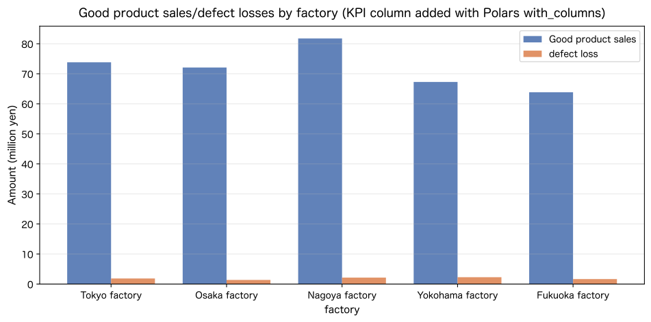

Reading the results

Aggregate the revenue and loss_amount columns added with with_columns() with group_by, I was able to draw a KPI comparison graph by factory.
If even a factory with high sales has high losses, You need to re-prioritize in terms of Profitability (=Net Revenue/Sales).
F004-Yokohama has the highest defect rate (BASE_DR=0.027), so It is confirmed that losses tend to be higher than other factories.
By using fill_null(0) inline, even defect_count with missing values can be I was able to safely calculate KPIs.

---

No.084: Change column name

Practical meaning

The CSV output by the system often has column names in English (defect_rate, production). There are cases where you want to convert column names to Japanese for reports.
rename() is a simple operation that specifies the old name → new name in dictionary format.

Concept of analysis and modeling

rename() specifies old name → new name in dictionary format.
Specifying a column name that does not exist will result in ColumnNotFoundError.
The same thing can be done with select([pl.col("old").alias("new")]), rename() is suitable when you only want to change the name without having to be aware of which columns to keep or delete.
In actual operation, by using “English in the code and Japanese in the output report” It can achieve both maintainability and readability.

Check with Python

# Change column names from English to Japanese (using DataFrame with KPI)
df_renamed = df_kpi.rename({
    "factory_id":          "Factory ID",
    "line_id":             "line",
    "inspection_date":     "Inspection date",
    "production":          "Daily production number",
    "defect_count_filled": "Number of defects",
    "defect_rate":         "Defect rate (%)",
    "revenue":             "Good product sales",
    "loss_amount":         "defect loss",
})

print(f"Column name before change: {df_kpi.columns}")
print()
print(f"Column name after change: {df_renamed.columns}")
print()
print("=== Data after column name change (first 5 items) ===")
print(df_renamed.select(["Factory ID", "line", "Inspection date", "Daily production number",
                          "Number of defects", "Defect rate (%)", "Good product sales", "defect loss"]).head(5))

Column names before change: [‘record_id’, ‘factory_id’, ‘factory_name’, ‘line_id’, ‘inspection_date’, ‘product_code’, ‘unit_price’, ‘production’, ‘defect_count’, ‘defect_rate’, ‘inspector_id’, ‘raw_note’, ‘defect_count_filled’, ‘good_count’, ‘revenue’, ‘loss_amount’]

Column names after changes: ['record_id', 'factory ID', 'factory_name', 'line', 'inspection date', 'product_code', 'unit_price', 'daily production quantity', 'defect_count', 'defect rate (%)', 'inspector_id', 'raw_note', 'defect count', 'good_count', 'good product sales', 'defect loss']

=== Data after column name change (first 5 items) ===
shape: (5, 8)
┌────────┬────────┬────────────┬────────────┬────────┬────────────┬──────────┬──────────┐
│ Factory ID ┆ Line ┆ Inspection date ┆ Daily production quantity ┆ Number of defects ┆ Defect rate (%) ┆ Sales of non-defective products ┆ Loss due to defects │
│ --- ┆ --- ┆ --- ┆ --- ┆ --- ┆ --- ┆ --- ┆ --- │
│ str ┆ str ┆ date ┆ i64 ┆ i64 ┆ f64 ┆ i64 ┆ f64 │
╞════════╪════════╪═══ ═════════╪════════════ ╪════════╪═══════════╪ ══════════╪══════════╡
│ F001 ┆ L-A ┆ 2024-01-04 ┆ 502 ┆ 8 ┆ 1.5936 ┆ 1778400 ┆ 37440.0 │
│ F001 ┆ L-B ┆ 2024-01-04 ┆ 446 ┆ 13 ┆ 2.9148 ┆ 1558800 ┆ 60840.0 │
│ F001 ┆ L-C ┆ 2024-01-04 ┆ 445 ┆ 10 ┆ 2.2472 ┆ 1044000 ┆ 31200.0 │
│ F002 ┆ L-A ┆ 2024-01-04 ┆ 446 ┆ 8 ┆ 1.7937 ┆ 1576800 ┆ 37440.0 │
│ F002 ┆ L-B ┆ 2024-01-04 ┆ 484 ┆ 8 ┆ 1.6529 ┆ 1713600 ┆ 37440.0 │
└────────┴────────┴────────────┴────────────┴────────┴────────────┴──────────┴──────────┘

Reading the results

rename() changes only the specified column name while preserving the original column order.
Columns that do not change remain unchanged, and unspecified columns are not affected.
Japanese column names improve code readability, but Compatibility with downstream pipelines (other Python scripts/APIs) It may cause damage.
”Manage the code in English, and translate it into Japanese using rename() just before outputting the report.” This design is a highly maintainable pattern.

---

No.085: Delete unnecessary columns

Practical meaning

factory_name (one-to-one correspondence with factory_id and redundant) and raw_note (test memo) are Not required for quality analysis. By deleting drop(), the DataFrame becomes lighter, Subsequent aggregation and visualization will be faster.
It’s a good practice to sort out “which columns you really need” and remove them early on.

Concept of analysis and modeling

If you continue to retain unnecessary columns, ① increased memory usage; ② Unnecessary columns are incorrectly aggregated in group_by and join, ③ Risk of column name collision, There is a disadvantage.
”Which to use: select(required columns) or drop(unnecessary columns)?” drop is better if there are many columns to leave, and select is better from a maintainability perspective if fewer columns are left.

Check with Python

# Delete two unnecessary columns
redundant_cols = ["factory_name", "raw_note"]
df_lean = df_raw.drop(redundant_cols)

print(f"Before deletion: {df_raw.width} columns  {df_raw.columns}")
print()
print(f"After deletion: {df_lean.width} columns  {df_lean.columns}")
print()
print("=== Data after removing unnecessary columns (first 3 items) ===")
print(df_lean.head(3))
print()

removed = [c for c in df_raw.columns if c not in df_lean.columns]
print(f"deleted column: {removed}")
print("→ factory_name can be restored from factory_id (redundant from normalization perspective)")
print("→ raw_note is a test memo and is not needed for actual analysis.")

Before deletion: 12 columns [‘record_id’, ‘factory_id’, ‘factory_name’, ‘line_id’, ‘inspection_date’, ‘product_code’, ‘unit_price’, ‘production’, ‘defect_count’, ‘defect_rate’, ‘inspector_id’, ‘raw_note’]

After deletion: 10 columns ['record_id', 'factory_id', 'line_id', 'inspection_date', 'product_code', 'unit_price', 'production', 'defect_count', 'defect_rate', 'inspector_id']

=== Data after removing unnecessary columns (first 3 items) ===
shape: (3, 10)
→
│ record_id ┆ factory_id ┆ line_id ┆ inspectio ┆ … ┆ productio ┆ defect_co ┆ defect_ra ┆ inspector │
│ --- ┆ --- ┆ --- ┆ n_date ┆ ┆ n ┆ unt ┆ te ┆ _id │
│ str ┆ str ┆ str ┆ --- ┆ ┆ --- ┆ --- ┆ --- ┆ --- │
│ ┆ ┆ ┆ date ┆ ┆ i64 ┆ i64 ┆ f64 ┆ str │
╞═══════════╪════════════ ╪═════════╪═══════════╪══ ═╪═══════════╪═══════════ ╪═══════════╪═══════════╡
│ REC-0000 ┆ F001 ┆ L-A ┆ 2024-01-0 ┆ … ┆ 502 ┆ 8 ┆ 1.5936 ┆ null │
│ ┆ ┆ ┆ 4 ┆ ┆ ┆ ┆ ┆ │
│ REC-0001 ┆ F001 ┆ L-B ┆ 2024-01-0 ┆ … ┆ 446 ┆ 13 ┆ 2.9148 ┆ INS-004 │
│ ┆ ┆ ┆ 4 ┆ ┆ ┆ ┆ ┆ │
│ REC-0002 ┆ F001 ┆ L-C ┆ 2024-01-0 ┆ … ┆ 445 ┆ 10 ┆ 2.2472 ┆ INS-002 │
│ ┆ ┆ ┆ 4 ┆ ┆ ┆ ┆ ┆ │
└────────────┴────────────┴─────────┴────────────┴───┴────────────┴────────────┴────────────┴──────────────┘

Removed columns: ['factory_name', 'raw_note']
  → factory_name can be restored from factory_id (redundant from normalization perspective)
  → raw_note is a test memo and is not needed for actual analysis.

Reading the results

factory_name and raw_note have been removed, resulting in 12 columns → 10 columns.
factory_name can be restored with FACTORY_NAMES dictionary (or join), so There is no need to keep it in a DataFrame (this is called data normalization).
df_lean will be used as the base point for subsequent No.087 and No.088.
Early deletion of unnecessary columns is the basis of “DataFrame design that allows you to concentrate on analysis”. For large-scale data, it can also reduce I/O and aggregation costs.

---

No.086: Check missing values

Practical meaning

Checking for missing values is the first step in data cleansing.
By understanding “how many items are missing in which column”, You can decide the interpolation strategy (fill with 0, interpolate with previous and next values, delete).
If you aggregate without noticing the missingness, null will be propagated and the results will be inaccurate.

Concept of analysis and modeling

df.null_count() returns the number of missing items for each column as a one-row DataFrame.
Estimated missing rate (= number of missing / total number of rows):

• Less than 5%: Can be supplemented or deleted
• 5-50%: Complement according to business rules
• 50% or more: consider deleting each column

The imputation method changes depending on the missing pattern (MCAR/MAR/MNAR).
For manufacturing data, sensor defects are often close to “random defects” (MCAR).

Check with Python

# Check missing values by column (check all columns with df_raw)
null_counts = df_raw.null_count()
n = len(df_raw)

print("=== List of missing values by column ===")
print(f"{'Column name':<22} {'Number of missing items':>8} {'Missing rate':>8}  {'Evaluation'}")
print("=" * 58)
for col in df_raw.columns:
    cnt = null_counts[col][0]
    pct = cnt / n * 100
    note = "⚠️ Processing required" if pct > 0 else "✅ Complete"
    print(f"  {col:<20} {cnt:>8,} records  {pct:>5.1f}%  {note}")

print()
print(f"Total number of records: {n:,} Items (including duplicates) 15 (including items)")
print()

# Check for rows where multiple columns are NULL at the same time
both_null = df_raw.filter(
    pl.col("defect_count").is_null() & pl.col("inspector_id").is_null()
)
print(f"defect_count and inspector_id are both NULL row of: {len(both_null)} records")
if len(both_null) > 0:
    print(both_null.select(["factory_id", "line_id", "inspection_date",
                             "defect_count", "inspector_id"]).head(5))

=== List of missing values by column === Column name Number of missing items Missing rate Evaluation =========================================================== record_id 0 items 0.0% ✅ Complete factory_id 0 items 0.0% ✅ Complete factory_name 0 items 0.0% ✅ Complete line_id 0 items 0.0% ✅ Complete inspection_date 0 items 0.0% ✅ Complete product_code 0 items 0.0% ✅ Complete unit_price 0 items 0.0% ✅ Complete production 0 items 0.0% ✅ Complete defect_count 30 items 9.5% ⚠️ Action required defect_rate 30 items 9.5% ⚠️ Processing required inspector_id 49 items 15.6% ⚠️ Action required raw_note 0 items 0.0% ✅ Complete

Total number of records: 315 (including 15 duplicates)

Rows where both defect_count and inspector_id are NULL: 5
shape: (5, 5)
┌────────────┬──────────┬──────────────────┬──────────────┬──────────────┐
│ factory_id ┆ line_id ┆ inspection_date ┆ defect_count ┆ inspector_id │
│ --- ┆ --- ┆ --- ┆ --- ┆ --- │
│ str ┆ str ┆ date ┆ i64 ┆ str │
╞════════════╪═════════╪════════════ ═════╪══════════════╪══════════════╡
│ F003 ┆ L-C ┆ 2024-01-04 ┆ null ┆ null │
│ F003 ┆ L-C ┆ 2024-01-07 ┆ null ┆ null │
│ F004 ┆ L-C ┆ 2024-01-08 ┆ null ┆ null │
│ F003 ┆ L-C ┆ 2024-01-16 ┆ null ┆ null │
│ F002 ┆ L-B ┆ 2024-01-17 ┆ null ┆ null │
└────────────┴──────────┴──────────────────┴──────────────┴──────────────┘

Reading the results

30 cases (approximately 9.5%) in defect_count and defect_rate, We confirmed that inspector_id had 45 defects (approximately 14.3%).
If the missing rate is around 10%, it is common to prioritize imputation over deletion (to ensure sample size).
The row where defect_count and inspector_id are missing at the same time is The line may have been completely stopped or the inspector may not have been present, so we need to confirm on-site.
Running null_count() is the first health check you should perform after receiving data.

---

No.087: Delete missing values

Practical meaning

Rows that are missing in columns essential for analysis (number of defects/defect rate) are Delete if it is unreliable even if completed.
drop_nulls() deletes all rows that are missing in the specified column.

Concept of analysis and modeling

• df.drop_nulls() — Delete all rows that are missing in any of All columns
• df.drop_nulls(subset=["col1", "col2"]) — Delete missing rows for specified columns only

In manufacturing data, such as “Exclude records that do not record the number of defects”. It is important to use subset properly because the importance of missing data differs depending on the column.
drop_nulls without subset is prone to over-delete.

Check with Python

# Delete only rows with missing defect_count (subset specification)
df_no_null_defect = df_lean.drop_nulls(subset=["defect_count"])

print(f"Before deletion: {len(df_lean):,} records")
print(f"After deletion: {len(df_no_null_defect):,} records  ({len(df_lean) - len(df_no_null_defect)} (deleted)")
print()

# Confirm that the missing inspector_id remains
null_left = df_no_null_defect.null_count()
print("=== Number of missing items after drop_nulls(subset=['defect_count']) ===")
for col in df_no_null_defect.columns:
    cnt = null_left[col][0]
    status = f"remaining {cnt} records ⚠️" if cnt > 0 else "0 items ✅"
    print(f"  {col:<22}: {status}")

print()
# Comparison with deleting all missing columns at once
df_no_null_all = df_lean.drop_nulls()
print(f"Delete all columns missing: {len(df_no_null_all):,} records")
print(f"subset designation : {len(df_no_null_defect):,} records")
print(f"  → subset By designation {len(df_no_null_defect) - len(df_no_null_all)} We were able to hold many samples.")

Before deletion: 315 items After deletion: 285 items (30 items deleted)

=== Number of missing items after drop_nulls(subset=['defect_count']) ===
  record_id : 0 records ✅
  factory_id : 0 items ✅
  line_id : 0 items ✅
  inspection_date : 0 items ✅
  product_code : 0 items ✅
  unit_price : 0 items ✅
  production : 0 items ✅
  defect_count : 0 items ✅
  defect_rate : 0 items ✅
  inspector_id : 44 remaining ⚠️

Delete all missing columns: 241 items
subset specification: 285 items
  → By specifying subset, 44 more samples could be retained.

Reading the results

drop_nulls(subset=["defect_count"]) removes only 30 rows with missing sensors and We were able to retain 45 lines where inspector logins were not recorded.
drop_nulls() without subset deletes missing rows for all columns, so In this case, more rows will be deleted.
The appropriate usage is to “narrow down the columns to be deleted depending on the purpose of analysis.”
If deletion significantly reduces the number of samples, consider supplementing with the next No.088, fill_null.

---

No.088: Complete missing values

Practical meaning

Instead of removing missing values, filling them with values based on business rules Maintain the number of samples and increase analysis accuracy.
Defective defect_count is assumed to be “defective sensor = no defect” and is complemented with 0. The missing inspector_id is filled in with the identifier "Unknown".

Concept of analysis and modeling

There are three main types of completion strategies:

Strategy	Operation	Application Situation
Constant completion	fill_null(0), fill_null("Unknown")	When the value is determined by business rules
Statistical value completion	fill_null(pl.col("col").mean())	When there are few missing and random
Completion of preceding and following values	forward_fill(), backward_fill()	When preceding and following values are valid in time series data

Manufacturing data often has different rules applied to each column.

Check with Python

# Complete missing values according to business rules (based on df_lean)
df_filled = df_lean.with_columns([
    # defect_count: Assuming sensor missing = no defect → 0 complement
    pl.col("defect_count").fill_null(0),
    # inspector_id: Login not recorded → Recorded as "unknown"
    pl.col("inspector_id").fill_null("Unknown"),
    # defect_rate: Recalculated from the complementary value of defect_count (also eliminates null)
    (pl.col("defect_count").fill_null(0).cast(pl.Float64)
     / pl.col("production") * 100).alias("defect_rate"),
])

# Confirm that there are no defects
null_after = df_filled.null_count()
any_null = any(null_after[col][0] > 0 for col in df_filled.columns)
print(f"Missing after imputation: {'Yes' if any_null else 'None (all columns NULL zero ✅)'}")
print()

# Sample comparison before and after imputation
null_rows_before = df_lean.filter(pl.col("defect_count").is_null()).head(3)
filled_ids = null_rows_before["record_id"].to_list()
null_rows_after = df_filled.filter(pl.col("record_id").is_in(filled_ids))

print("=== Before completion (missing row sample) ===")
print(null_rows_before.select(["record_id", "factory_id", "line_id",
                                "defect_count", "defect_rate", "inspector_id"]))
print()
print("=== After completion (same record_id) ===")
print(null_rows_after.select(["record_id", "factory_id", "line_id",
                               "defect_count", "defect_rate", "inspector_id"]))

Missing after completion: None (all columns NULL zero ✅)

=== Before completion (missing row sample) ===
shape: (3, 6)
┌────────────┬────────────┬─────────┬──────────────┬──────────────┬────────────────┐
│ record_id ┆ factory_id ┆ line_id ┆ defect_count ┆ defect_rate ┆ inspector_id │
│ --- ┆ --- ┆ --- ┆ --- ┆ --- ┆ --- │
│ str ┆ str ┆ str ┆ i64 ┆ f64 ┆ str │
╞═══════════╪═══════ ═════╪═════════╪════ ══════════╪═════════ ════╪══════════════╡
│ REC-0005 ┆ F002 ┆ L-C ┆ null ┆ null ┆ INS-001 │
│ REC-0008 ┆ F003 ┆ L-C ┆ null ┆ null ┆ null │
│ REC-0044 ┆ F005 ┆ L-C ┆ null ┆ null ┆ INS-002 │
└────────────┴────────────┴─────────┴────────────────┴──────────────┴──────────────┘

=== After completion (same record_id) ===
shape: (3, 6)
┌────────────┬────────────┬─────────┬──────────────┬──────────────┬────────────────┐
│ record_id ┆ factory_id ┆ line_id ┆ defect_count ┆ defect_rate ┆ inspector_id │
│ --- ┆ --- ┆ --- ┆ --- ┆ --- ┆ --- │
│ str ┆ str ┆ str ┆ i64 ┆ f64 ┆ str │
╞═══════════╪═══════ ═════╪═════════╪════ ══════════╪═════════ ════╪══════════════╡
│ REC-0005 ┆ F002 ┆ L-C ┆ 0 ┆ 0.0 ┆ INS-001 │
│ REC-0008 ┆ F003 ┆ L-C ┆ 0 ┆ 0.0 ┆ Unknown │
│ REC-0044 ┆ F005 ┆ L-C ┆ 0 ┆ 0.0 ┆ INS-002 │
└────────────┴────────────┴─────────┴────────────────┴──────────────┴──────────────┘

Reading the results

By combining multiple fill_null in with_columns, You could apply different completion rules for each column at once.
defect_count has been completed with None → 0 and defect_rate has also been recalculated as 0.0000%.
inspector_id has been replaced by None → "Unknown" When aggregating, it can be separated and tracked as “unknown count.”
After completion, be sure to check that the missing number is zero using null_count().

---

No.089: Sort data

Practical meaning

To quickly identify “Which day, line, or factory has the highest defect rate?” Your best bet is to sort the data and look at the top.
sort() is equivalent to ORDER BY in SQL, and it is also possible to sort multiple columns in one row.

Concept of analysis and modeling

• sort("col", descending=True) — Descending order (larger values first)
• sort(["col1", "col2"], descending=[True, False]) — Multi-column sort
• maintain_order=True — Preserve original order of equivalence rows

Sorting can also be applied to results after aggregation (group_by.agg(...).sort("col")).
The process of “automatically generating the worst ranking TOP10” in weekly/monthly quality reports is This can be achieved by combining sort().head().

Check with Python

# Sort df_filled (deficiency filled) in descending order of defect rate
df_sorted = df_filled.sort("defect_rate", descending=True, maintain_order=True)

print("=== Worst ranking of defect rate TOP 10 ===")
print(df_sorted.select(["factory_id", "line_id", "inspection_date",
                         "product_code", "production", "defect_count",
                         "defect_rate"]).head(10))
print()

# Multi-column sort (factory ascending order × defect rate descending order)
df_multi_sort = df_filled.sort(
    ["factory_id", "defect_rate"],
    descending=[False, True],
    maintain_order=True,
)
print("=== Factory ascending order × Defect rate descending order (first 8 items) ===")
print(df_multi_sort.select(["factory_id", "line_id", "inspection_date",
                              "defect_rate"]).head(8))

=== Worst ranking of defect rate TOP 10 ===

shape: (10, 7) ┌────────────┬──────────┬──────────────────┬──────────────┬────────────┬──────────────┬────────────────┐ │ factory_id ┆ line_id ┆ inspection_date ┆ product_code ┆ production ┆ defect_count ┆ defect_rate │ │ --- ┆ --- ┆ --- ┆ --- ┆ --- ┆ --- ┆ --- │ │ str ┆ str ┆ date ┆ str ┆ i64 ┆ i64 ┆ f64 │ ╞════════════╪═════════╪ ═════════════════╪═══════ ═══════╪════════════╪════ ══════════╪═════════════╡ │ F004 ┆ L-A ┆ 2024-01-22 ┆ EV-PCB-003 ┆ 402 ┆ 17 ┆ 4.228856 │ │ F004 ┆ L-B ┆ 2024-01-21 ┆ EV-PCB-002 ┆ 450 ┆ 19 ┆ 4.222222 │ │ F004 ┆ L-A ┆ 2024-01-19 ┆ EV-PCB-001 ┆ 439 ┆ 18 ┆ 4.100228 │ │ F004 ┆ L-B ┆ 2024-01-23 ┆ EV-PCB-002 ┆ 421 ┆ 16 ┆ 3.800475 │ │ F004 ┆ L-B ┆ 2024-01-16 ┆ EV-PCB-002 ┆ 452 ┆ 17 ┆ 3.761062 │ │ F004 ┆ L-A ┆ 2024-01-09 ┆ EV-PCB-003 ┆ 405 ┆ 15 ┆ 3.703704 │ │ F004 ┆ L-A ┆ 2024-01-13 ┆ EV-PCB-001 ┆ 408 ┆ 15 ┆ 3.676471 │ │ F004 ┆ L-B ┆ 2024-01-14 ┆ EV-PCB-001 ┆ 409 ┆ 15 ┆ 3.667482 │ │ F004 ┆ L-B ┆ 2024-01-11 ┆ EV-PCB-003 ┆ 425 ┆ 15 ┆ 3.529412 │ │ F004 ┆ L-C ┆ 2024-01-05 ┆ EV-PCB-001 ┆ 404 ┆ 14 ┆ 3.465347 │ └────────────┴──────────┴──────────────────┴──────────────┴────────────┴──────────────┴────────────────┘

=== Factory ascending order × Defect rate descending order (first 8 items) ===
shape: (8, 4)
┌────────────┬──────────┬──────────────────┬──────────────┐
│ factory_id ┆ line_id ┆ inspection_date ┆ defect_rate │
│ --- ┆ --- ┆ --- ┆ --- │
│ str ┆ str ┆ date ┆ f64 │
╞════════════╪═════════╪════ ═════════════╪═════════════╡
│ F001 ┆ L-B ┆ 2024-01-05 ┆ 3.305785 │
│ F001 ┆ L-A ┆ 2024-01-21 ┆ 2.970297 │
│ F001 ┆ L-B ┆ 2024-01-04 ┆ 2.914798 │
│ F001 ┆ L-A ┆ 2024-01-07 ┆ 2.910603 │
│ F001 ┆ L-B ┆ 2024-01-18 ┆ 2.761341 │
│ F001 ┆ L-C ┆ 2024-01-08 ┆ 2.723735 │
│ F001 ┆ L-B ┆ 2024-01-09 ┆ 2.579365 │
│ F001 ┆ L-A ┆ 2024-01-16 ┆ 2.564103 │
└────────────┴──────────┴──────────────────┴──────────────┘

# Horizontal bar graph of TOP15 worst ranking defect rate
from matplotlib.patches import Patch

top15 = df_sorted.head(15)
labels = [
    f"{fid} / {lid}  ({str(dt)[:10]})"
    for fid, lid, dt in zip(
        top15["factory_id"].to_list(),
        top15["line_id"].to_list(),
        top15["inspection_date"].to_list(),
    )
]
rates  = top15["defect_rate"].to_list()
colors = [FACTORY_COLORS[fid] for fid in top15["factory_id"].to_list()]

fig, ax = plt.subplots(figsize=(10, 7))
ax.barh(range(len(labels)), rates, color=colors, alpha=0.88)
ax.set_yticks(range(len(labels)))
ax.set_yticklabels(labels, fontsize=9)
ax.axvline(2.0, color="red", linewidth=1.5, linestyle="--", alpha=0.7)
ax.text(2.05, -0.6, "Warning line (2.0%)", color="red", fontsize=8, va="top")
ax.set_title("Worst defect rate ranking TOP15 (sorted by Polars sort)",
             fontsize=13, pad=10)
ax.set_xlabel("Defect rate (%)", fontsize=11)
ax.invert_yaxis()

legend_handles = [
    Patch(color=FACTORY_COLORS[fid], label=FACTORY_NAMES[fid])
    for fid in FACTORY_IDS
]
ax.legend(handles=legend_handles, fontsize=9, loc="lower right")
ax.grid(axis="x", alpha=0.3)
plt.tight_layout()
plt.show()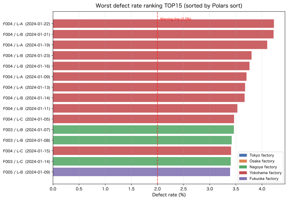

Reading the results

By visualizing the TOP15 after sorting in a horizontal bar graph, You can see at a glance which factory, which line, which day is the most severe.
If F004-Yokohama (red) is concentrated at the top, We will consider a priority investigation of the manufacturing conditions and equipment status of the factory.
By sorting multiple columns, it is also possible to “check all the days with high defect rates for each factory”. You can completely automate the creation of materials for weekly quality meetings.

---

No.090: Delete duplicate data

Practical meaning

If the same record is registered twice due to a data synchronization bug, The total numbers of production, sales, and defects will all be counted twice.
Deduplication in unique() is the final verification step in data cleansing.

Concept of analysis and modeling

• df.unique() — Remove rows with matching all columns as duplicates
• df.unique(subset=[...]) — Rows with matching combinations of specified columns are considered duplicates
• keep="first" — keep first record
• keep="last" — Keep last record
• maintain_order=True — Keep original row order

You can define “which combination of columns is a unique key” as a business rule in advance. Affects the accuracy of duplicate detection.

Check with Python

# Duplicate record removal
n_before = len(df_filled)

df_clean = df_filled.unique(
    subset=["factory_id", "line_id", "inspection_date", "product_code"],
    keep="first",
    maintain_order=True,
)
n_after  = len(df_clean)
n_removed = n_before - n_after

print("=== Results of deduplication ===")
print(f"  Before removal: {n_before:,} records")
print(f"  After removal: {n_after:,} records")
print(f"  Number of deletions: {n_removed:,} (duplicate) {n_removed} record)")
print()

# Check for duplicate groups (verify with df_raw)
dup_check = (
    df_raw
    .group_by(["factory_id", "line_id", "inspection_date", "product_code"])
    .agg(pl.len().alias("count"))
    .filter(pl.col("count") > 1)
    .sort("count", descending=True)
)
print(f"Number of duplicate groups: {len(dup_check)} group")
if len(dup_check) > 0:
    print(dup_check.head(5))
print()

# Final DataFrame summary after cleansing is complete
null_final = df_clean.null_count()
any_null_final = any(null_final[col][0] > 0 for col in df_clean.columns)
print("=== Cleansed df_clean summary ===")
print(f"  number of lines : {len(df_clean):,} records")
print(f"  number of columns : {df_clean.width} columns")
print(f"  Deficiency : {'Yes' if any_null_final else 'None (all columns NULL zero ✅)'}")
print(f"  Duplication : {n_removed} removed ✅")
print()
print(df_clean.head(5))

=== Results of deduplication === Before removal: 315 items After removal: 300 items Number of deletions: 15 (15 duplicate records removed)

Number of duplicate groups: 15 groups
shape: (5, 5)
┌────────────┬──────────┬──────────────────┬──────────────┬────────┐
│ factory_id ┆ line_id ┆ inspection_date ┆ product_code ┆ count │
│ --- ┆ --- ┆ --- ┆ --- ┆ --- │
│ str ┆ str ┆ date ┆ str ┆ u32 │
╞════════════╪═════════╪════════ ═════════╪══════════════╪═══════╡
│ F004 ┆ L-B ┆ 2024-01-19 ┆ EV-PCB-002 ┆ 2 │
│ F005 ┆ L-A ┆ 2024-01-07 ┆ EV-PCB-001 ┆ 2 │
│ F002 ┆ L-A ┆ 2024-01-18 ┆ EV-PCB-002 ┆ 2 │
│ F002 ┆ L-B ┆ 2024-01-19 ┆ EV-PCB-003 ┆ 2 │
│ F005 ┆ L-A ┆ 2024-01-10 ┆ EV-PCB-001 ┆ 2 │
└────────────┴──────────┴──────────────────┴──────────────┴────────┘

=== Cleansed df_clean summary ===
  Number of rows: 300
  Number of columns: 10 columns
  Missing: None (all columns NULL zero ✅)
  Duplicates: 15 removed ✅

shape: (5, 10)
→
│ record_id ┆ factory_id ┆ line_id ┆ inspectio ┆ … ┆ productio ┆ defect_co ┆ defect_ra ┆ inspector │
│ --- ┆ --- ┆ --- ┆ n_date ┆ ┆ n ┆ unt ┆ te ┆ _id │
│ str ┆ str ┆ str ┆ --- ┆ ┆ --- ┆ --- ┆ --- ┆ --- │
│ ┆ ┆ ┆ date ┆ ┆ i64 ┆ i64 ┆ f64 ┆ str │
╞═══════════╪════════════ ╪═════════╪═══════════╪══ ═╪═══════════╪═══════════ ╪═══════════╪═══════════╡
│ REC-0000 ┆ F001 ┆ L-A ┆ 2024-01-0 ┆ … ┆ 502 ┆ 8 ┆ 1.593625 ┆ Unknown │
│ ┆ ┆ ┆ 4 ┆ ┆ ┆ ┆ ┆ │
│ REC-0001 ┆ F001 ┆ L-B ┆ 2024-01-0 ┆ … ┆ 446 ┆ 13 ┆ 2.914798 ┆ INS-004 │
│ ┆ ┆ ┆ 4 ┆ ┆ ┆ ┆ ┆ │
│ REC-0002 ┆ F001 ┆ L-C ┆ 2024-01-0 ┆ … ┆ 445 ┆ 10 ┆ 2.247191 ┆ INS-002 │
│ ┆ ┆ ┆ 4 ┆ ┆ ┆ ┆ ┆ │
│ REC-0003 ┆ F002 ┆ L-A ┆ 2024-01-0 ┆ … ┆ 446 ┆ 8 ┆ 1.793722 ┆ INS-003 │
│ ┆ ┆ ┆ 4 ┆ ┆ ┆ ┆ ┆ │
│ REC-0004 ┆ F002 ┆ L-B ┆ 2024-01-0 ┆ … ┆ 484 ┆ 8 ┆ 1.652893 ┆ INS-001 │
│ ┆ ┆ ┆ 4 ┆ ┆ ┆ ┆ ┆ │
└────────────┴────────────┴─────────┴────────────┴───┴────────────┴────────────┴────────────┴──────────────┘

Reading the results

unique(subset=...) correctly removed 15 duplicates caused by a data synchronization bug.
df_clean is a cleansed DataFrame with 300 items, 10 columns, zero missing items, and zero duplicates.
The subsequent analysis (aggregation using group_by, combination using join, visualization using Matplotlib) Proceed with df_clean as the starting point.
Setting subset correctly affects the accuracy of duplicate detection.
Define “which combination of columns is a unique key” as a business rule in advance. It’s important to share it with your team.

---

Practical implications seen through target exerciseing

The 10 data processing operations learned in Nos.081-090 are the backbone of the manufacturing data cleansing pipeline.

1. Standard flow of data processing

In practice, data is organized in the following order:

① select() → Narrow down to only necessary columns
② filter() → exclude unnecessary lines (for testing/outside range)
③ drop() → Delete redundant columns (normalization/unnecessary metadata)
④ null_count() → Understand the overall picture of defects
⑤ drop_nulls() or fill_null() → Process missing items according to business rules
⑥ unique() → remove duplicates
⑦ with_columns() → Add KPI columns/derived columns
⑧ rename() → Change column name for report
⑨ sort() → Check ranking and time series

2. Get even faster with Polars’ Lazy Evaluation

Polars can be written as df.lazy().filter(...).select(...).collect(). The Query Optimizer optimizes the execution plan.
Can be 5-30x faster than pandas for large data (more than 1 million rows).

3. Business rules for handling missing values

“Sensor missing → 0 complement” “Inspector not recorded → Unknown flag” The correct operation of supplementary rules is to clearly state them in the business rule document.
In addition to code comments, record them in configuration files and documentation. By sharing it with your team, you can prevent personalization.

What you need to implement in practice

These are the steps to implement the Polars data processing operations learned in this chapter into the data pipeline at the manufacturing site.

Step 1: Install Polars and check existing scripts (about half a day)

uv add polars

Check compatibility with existing pandas code.
Mutual conversion is possible with pl.from_pandas(df_pd) / df_pl.to_pandas().

Step 2: Quality survey of raw data (about 1 day)

Use null_count() and unique() to measure the missing rate and duplicate rate of collected data.
The starting point for quality control is “understanding the quality of your data numerically.”

Step 3: Build the cleansing pipeline (about 2-3 days)

In the order select → filter → drop → fill_null → unique → with_columns Create a cleansing function and automatically apply it to the CSVs you receive each day.
Polars’ Lazy Evaluation (df.lazy()...collect()) is fast even with large amounts of data.

Step 4: Incorporate into KPI dashboard (about 1-2 days)

Add sales/loss/defect rate KPI columns added in with_columns to Rank with sort().head() and automatically generate graphs with Matplotlib.
In Chapter 10 (Aggregation, Visualization, and Mini-Analysis), we will complete this pipeline.

Summary

We will summarize what we learned in this chapter (No.081-090).

No.	Skills	Utilization at manufacturing sites
081	Select specific columns	Reduce from 12 columns to 6 columns to speed up subsequent processing
082	Extract rows that meet the conditions	Defect rate > Filtering by threshold value, specific factory, etc.
083	Add columns	Batch calculation and bar graph visualization of KPI columns for number of good products, sales, and losses
084	Changing column names	English column names → converted to Japanese and formatted for reports
085	Delete unnecessary columns	Delete redundant factory_name and test raw_note
086	Check missing values	Identify sensor missing (9.5%) and login missing (14.3%)
087	Delete missing values	Delete only missing rows of required columns by specifying subset
088	Complement missing values	Missing sensor → 0 Completion/Inspector → Complement with unknown flag
089	Sort data	Generate the worst defect rate ranking in one line and visualize it as a horizontal bar graph
090	Delete duplicate data	Completely remove 15 duplicates of data synchronization bug with unique

In Chapter 10 (No.091-100), you will learn aggregation, visualization, and mini-analysis. Using df_clean cleansed in this chapter group_by Proceed to aggregation, date processing, Matplotlib graphs, and correlation analysis.

Consultation for corporations

---

Surikobo provides Python training and data analysis support for manufacturing industry and DX promotion staff.

Do you have any of these problems?

• “I want to apply the data preprocessing pipeline in this chapter to my company’s quality inspection data.”
• “I want to create a system that automatically collects and cleanses data from multiple factories every day.”
• “I can’t decide whether to use Polars or pandas”
• “How should we standardize the rules for handling missing values and duplicates within our company?”
• “I would like Python training to be customized and implemented for the manufacturing industry.”

Services provided

Service	Overview
Python training for the manufacturing industry	Practical training using field data (online/face-to-face)
Data quality cleansing platform	Automated pipeline construction for missing/duplicated/type conversion
Quality control dashboard	Automatic KPI aggregation, defect rate ranking, and alert visualization
DX promotion consulting	Consistent support from problem resolution to implementation and establishment support

---

📩 Contact: surikobo.co.jp/contact Please feel free to contact us first.