Introduction to Polars: Interpret production line data quickly and safely

100 Exercises Chapter 8 (No.071-No.080): Introduction to Polars

This article is Chapter 8 of the “100 Exercises on Introduction to Python for Data Analysis” series.
In Chapter 7 (No.061-070), we learned array operations using NumPy.
This chapter uses Polars - a next-generation DataFrame library that is faster and more memory efficient than pandas. Learn the basic operations for reading, checking, and aggregating monthly production results data at electronic parts factories.

[!NOTE] This material is a notebook that has been used by Surikobo (or its representative, Hiroshi Wayama) in corporate training in the past. Reorganized and edited with permission from the company and published.
All published data is fictitious and has no relation to actual companies, factories, or numbers.

Introduction: Practical issues in the manufacturing industry covered in this article

This is the first work of the month for Mr. K, a member of the production management team at an electronic parts manufacturing factory (printed circuit board mounting line).

Regular work at the beginning of every month
  1. Export the daily production results CSV of 5 lines from the management system (20 business days x 5 lines)
  2. Open the CSV in Excel and visually check the number of rows and columns (“How many rows are there this month?”)
  3. Manually check whether the data type of each column is correct (Is the date a string?)
  4. Manual calculation of basic statistics (average, maximum, minimum, standard deviation) using functions
  5. Visually scroll to find days with abnormally low production numbers or missing days

Using Python’s Polars, Load CSV with tens of thousands of rows up to 5x faster than pandas, Type checking, statistics, and abnormal value detection can be completed with 3 to 5 lines of code.

Common situations in the field

Scene	Task
CSV loading is slow	Reading one month’s worth of CSV (tens of thousands of lines) using pandas feels slow
Type mismatch	Aggregation is not possible as the date column is object (character string)
Check column names	Check “What column is this column?” every time in Excel
Understand the number of rows	Check if there are any missing days by visually scrolling
Checking the statistics	Unable to interpret and utilize the results of describe()

“5 things to check first after reading the data” - Number of rows, number of columns, column names, types, statistics - You will systematically learn this in this chapter.

Why is this problem difficult to judge?

Polars is similar to pandas, with some important differences.

1. df["Column name"] vs df.select("Column name") df["Column name"] returns pl.Series, while df.select("Column name") returns pl.DataFrame.
   It is necessary to use them properly depending on the purpose.

2. Difference between Eager mode and Lazy mode pl.read_csv() is in Eager mode that runs immediately.
   Lazy mode of pl.scan_csv() → .collect() is efficient for large-scale data.
   This chapter covers Eager mode as the basis.

3. Return value of describe() is DataFrame Polars’ describe() returns DataFrame.
   Since statistics including non-numeric type columns are displayed, it is necessary to check the column types first.

4. Difference between null and NaN In Polars, missing values are represented as null (=None in Python).
   NaN is separately distinguished as a floating point special value.

Overall picture of the exercises covered in this chapter

No.	Title	Usage in manufacturing industry
071	Understanding the role of Polars	Sorting out the differences with pandas and determining whether it can be applied to large-scale manufacturing data
072	Import Polars	Import, version confirmation, and basic settings
073	Creating a Series	Handling single column data such as number of defects and number of production
074	Create a DataFrame	Build a production results table by line
075	Load CSV as DataFrame	Load monthly production results CSV and basic check
076	Check the first and last lines	Visual check immediately after loading (head/tail)
077	Check the number of rows and columns	Check for missing dates and extra rows (shape)
078	Check column names	Check and normalize column name list
079	Check the data type	Check the correct type for date and numeric types
080	Check the basic statistics	Check the average, maximum, minimum, and standard deviation of production quantity and defect rate at once

Preparing the Python environment

import subprocess, sys

res = subprocess.run(["sw_vers", "-productVersion"], capture_output=True, text=True)
print(f"macOS : {res.stdout.strip()}")
print(f"Python: {sys.version}")

macOS : 26.3
Python: 3.11.9 (main, Apr 19 2024, 11:43:47) [Clang 14.0.6 ]

import numpy as np
import polars as pl
import matplotlib
import matplotlib.pyplot as plt
import csv, os, datetime

matplotlib.rcParams['font.family'] = 'Hiragino Maru Gothic Pro'
%config InlineBackend.figure_format = 'svg'
np.random.seed(42)

print("Library loading completed")
print(f"  NumPy     : {np.__version__}")
print(f"  Polars    : {pl.__version__}")
print(f"  Matplotlib: {matplotlib.__version__}")

Library loading completed NumPy: 1.26.4 Polars: 1.42.1 Matplotlib: 3.9.2

Creation of fictitious data

Assumed scenario: Electronic parts manufacturing factory / Printed circuit board mounting line Production management team Period: January 2024 (20 business days) Management target: 5 product lines (different board types, unit prices, and standard failure rates) Output: Monthly production results CSV (production_jan2024.csv)

# settings
np.random.seed(42)
LINE_IDS   = ["PCB-A1", "PCB-A2", "PCB-B1", "PCB-B2", "PCB-C1"]
LINE_NAMES = {
    "PCB-A1": "Substrate A-Small", "PCB-A2": "Board A-Medium size",
    "PCB-B1": "Board B-Small", "PCB-B2": "Substrate B-High Density", "PCB-C1": "Substrate C-Large",
}
BASE_PROD = {"PCB-A1": 480, "PCB-A2": 360, "PCB-B1": 520, "PCB-B2": 280, "PCB-C1": 200}
BASE_DR   = {"PCB-A1": 0.018, "PCB-A2": 0.022, "PCB-B1": 0.015, "PCB-B2": 0.031, "PCB-C1": 0.025}
UNIT_PRICE = {"PCB-A1": 850, "PCB-A2": 1200, "PCB-B1": 760, "PCB-B2": 2400, "PCB-C1": 3200}

# Business days in January 2024 (Monday to Friday, 20 days)
biz_days, d = [], datetime.date(2024, 1, 4)
while len(biz_days) < 20:
    if d.weekday() < 5:
        biz_days.append(d)
    d += datetime.timedelta(days=1)

# data generation
records = []
for date in biz_days:
    for line in LINE_IDS:
        prod     = max(10, int(np.random.normal(BASE_PROD[line], BASE_PROD[line] * 0.05)))
        dr       = max(0.0, np.random.normal(BASE_DR[line], 0.005))
        defects  = int(prod * dr)
        work_h   = round(min(9.0, max(6.0, np.random.normal(7.8, 0.3))), 1)
        machine  = f"M{LINE_IDS.index(line)+1:02d}-{np.random.randint(1, 4)}"
        records.append({
            "date": date.strftime("%Y-%m-%d"),
            "line": line,
            "line_name": LINE_NAMES[line],
            "production_count": prod,
            "defect_count": defects,
            "working_hours": work_h,
            "unit_price": UNIT_PRICE[line],
            "machine_id": machine,
        })

# CSV save
CSV_PATH = "production_jan2024.csv"
with open(CSV_PATH, "w", newline="", encoding="utf-8") as f:
    writer = csv.DictWriter(f, fieldnames=records[0].keys())
    writer.writeheader()
    writer.writerows(records)

print(f"Generation completed: {CSV_PATH}")
print(f"  Number of records : {len(records):,} rows")
print(f"  number of columns       : {len(records[0])} columns")
print(f"  period       : {records[0]['date']} ~ {records[-1]['date']}")
print(f"  Number of lines   : {len(LINE_IDS)} line")

Generation completed: production_jan2024.csv Number of records: 100 lines Number of columns: 8 columns Period: 2024-01-04 ~ 2024-01-31 Number of lines: 5 lines

---

No.071: Understand the role of Polars

Practical meaning

Production performance data at manufacturing sites is accumulated every day, and over several months it reaches tens of thousands to hundreds of thousands of lines.
Although traditional pandas is sufficient, Polars is faster and more memory efficient than pandas. Suitable for DX infrastructure in the manufacturing industry, which requires the ability to handle large-scale data.

Criteria for choosing Polars:

• Processing target is more than 100,000 lines
• Repeated automatic execution of aggregation and filtering processes (daily batch processing, etc.)
• Situations where multiple data sources are combined and analyzed

Concept of analysis and modeling

Polars uses columnar storage based on the Apache Arrow format.
Column-by-column operations such as “total only defective number columns” are particularly fast.

Comparison items	pandas	Polars
Base format	NumPy	Apache Arrow
Speed (large scale)	Standard	Up to 5 times more
Memory usage	High	Low
Missing value type	NaN (float)	null (type independent)
Lazy evaluation (Lazy)	None	Yes (scan_csv → collect)

Check with Python

# Polars version check and main class list
print(f"Polars version: {pl.__version__}")
print()

# Main class confirmation
for cls in ["DataFrame", "Series", "LazyFrame", "Expr"]:
    print(f"  pl.{cls}")
print()

# Easily measure DataFrame creation time while changing the number of rows
import time

print(f"{'number of lines':>10s}  {'Polars creation time (ms)':>22s}")
print("-" * 38)
for n in [1_000, 10_000, 100_000]:
    data = {"val": list(range(n))}
    t0 = time.perf_counter()
    _ = pl.DataFrame(data)
    t1 = time.perf_counter()
    print(f"{n:>10,d}  {(t1 - t0) * 1000:>20.3f} ms")

Polars version: 1.42.1

  pl.DataFrame
  pl.Series
  pl.LazyFrame
  pl.Expr

        Number of rows Polars creation time (ms)
--------------------------------------
     1,000 2.601ms
    10,000 0.881ms
   100,000 0.622ms

Reading the results

• Polars is fast even on small data, but the advantage becomes more pronounced as the number of rows increases.
• If you do monthly or yearly batch aggregation on the manufacturing floor, it’s worth considering migrating to Polars.
• Four classes are the core of Polars: DataFrame, Series, LazyFrame, Expr.

---

No.072: Import Polars

Practical meaning

Correct import of libraries is the starting point for analysis.
The habit of explicitly checking versions is important during team development and when moving to production. This is important to prevent the problem of “it was working but suddenly stops working”.

Concept of analysis and modeling

Polars has a well-established convention of import polars as pl (corresponds to pandas’ pd).
requirements.txt for manufacturing data analysis project Fixing the version like polars>=1.0 will improve reproducibility.

Check with Python

# Import Polars and check version
import polars as pl
import sys

print("=" * 42)
print("Checking the execution environment")
print("=" * 42)
print(f"  Python    : {sys.version.split()[0]}")
print(f"  Polars    : {pl.__version__}")
print(f"  NumPy     : {np.__version__}")
print(f"  Matplotlib: {matplotlib.__version__}")
print("=" * 42)
print()

# Checking typical import styles
print("Recommended import style:")
print("import polars as pl # Polars body")
print("from polars import col, lit # When using frequently used functions in short form")

=========================================== Checking the execution environment =========================================== Python: 3.11.9 Polars: 1.42.1 NumPy: 1.26.4 Matplotlib: 3.9.2 ===========================================

Recommended import style:
  import polars as pl # Polars body
  from polars import col, lit # When using frequently used functions in short form

Reading the results

• You can check the version with pl.__version__.
• By recording the execution environment at the beginning of the project, You can track “in which environment it was executed” later.
• Polars’ API changes more frequently than pandas, so version fixing is especially important.

---

No.073: Create Series

Practical meaning

Series is a basic Polars data structure that represents one column (one-dimensional data).
At the manufacturing site, things like list of defective items on all lines on a given day'' and list of average operating rates for 5 lines”, etc. Used to manage single indicators collectively.

Concept of analysis and modeling

It is recommended to explicitly type when creating pl.Series.
Polars is good at type inference, but in manufacturing data, integer/floating point distinctions affect aggregation results.

Polars type	Application in manufacturing data
Int32 / Int64	Production quantity, defective quantity (integer)
Float64	Defect rate, operating rate (decimal)
String	Line name, device ID
Date	Production date

Check with Python

# Number of defects per day for 5 lines Series
defect_s = pl.Series("defect_count", [8, 12, 5, 18, 7], dtype=pl.Int32)
print("Defective number Series:")
print(defect_s)
print()

# Occupancy rate Series
avail_s = pl.Series(
    "availability_rate",
    [0.952, 0.881, 0.975, 0.843, 0.921],
    dtype=pl.Float64,
)
print("Occupancy rate Series:")
print(avail_s)
print()

# Series attributes
print("Series attribute:")
print(f"  name   : {defect_s.name}")
print(f"  mold     : {defect_s.dtype}")
print(f"  Number of elements : {len(defect_s)}")
print()

# Basic operations
print("Basic statistics for number of defects Series:")
print(f"  Total  : {defect_s.sum()}")
print(f"  average  : {defect_s.mean():.2f}")
print(f"  maximum  : {defect_s.max()}")
print(f"  minimum  : {defect_s.min()}")

Defective number Series: shape: (5,) Series: ‘defect_count’ [i32] [ 8 12 5 18 7 ]

Occupancy rate Series:
shape: (5,)
Series: 'availability_rate' [f64]
[
	0.952
	0.881
	0.975
	0.843
	0.921
]

Series attribute:
  Name: defect_count
  Type: Int32
  Number of elements: 5

Basic statistics for number of defects Series:
  Total : 50
  Average: 10.00
  Max: 18
  Minimum: 5

Reading the results

• By specifying dtype for pl.Series, errors due to type mismatch can be prevented.
• .sum(), .mean(), .max(), .min() can be called directly, Operations such as “instantly check the total number of defects on 5 lines” can be written concisely.
• From the total number of defects 50, we can see that 50 defective products occurred in the past day.
  PCB-B2 has the highest number of defects, 18, and can be said to be a line that requires priority management.

---

No.074: Create a DataFrame

Practical meaning

DataFrame is tabular data with multiple columns.
At the manufacturing site, “line names, production numbers, defective numbers, and operating rates are summarized in one table” This is the basic operation.

Concept of analysis and modeling

Main methods of creating DataFrame:

1. Created from a dictionary (The simplest and most suitable for validating fictitious data)
2. Create from Series list
3. Load from CSV/Parquet file (handled in No.075)

Check with Python

# 5 line production results on January 4, 2024 (first business day) DataFrame
df_day1 = pl.DataFrame({
    "line":             ["PCB-A1", "PCB-A2", "PCB-B1", "PCB-B2", "PCB-C1"],
    "line_name":        ["Substrate A-Small", "Board A-Medium size", "Board B-Small", "Substrate B-High Density", "Substrate C-Large"],
    "production_count": [472, 351, 515, 274, 198],
    "defect_count":     [8,   12,  5,   18,  7],
    "working_hours":    [7.8, 8.1, 7.6, 7.9, 8.0],
    "unit_price":       [850, 1200, 760, 2400, 3200],
})

print("January 4, 2024 Production Results DataFrame:")
print(df_day1)
print()

# Type of each column
print("Data type for each column:")
for col, dtype in zip(df_day1.columns, df_day1.dtypes):
    print(f"  {col:22s}: {dtype}")
print()

# Add defect rate column (preparation for adding column)
df_day1_ext = df_day1.with_columns(
    (pl.col("defect_count") / pl.col("production_count") * 100)
    .round(2)
    .alias("defect_rate_pct")
)
print("Defect rate (%) After adding:")
print(df_day1_ext.select(["line", "production_count", "defect_count", "defect_rate_pct"]))

January 4, 2024 Production Results DataFrame: shape: (5, 6) ┌────────┬──────────────┬──────────────────┬──────────────┬────────────────┬────────────┐ │ line ┆ line_name ┆ production_count ┆ defect_count ┆ working_hours ┆ unit_price │ │ --- ┆ --- ┆ --- ┆ --- ┆ --- ┆ --- │ │ str ┆ str ┆ i64 ┆ i64 ┆ f64 ┆ i64 │ ╞════════╪════════════ ══╪══════════════════╪ ══════════════╪═══════ ════════╪════════════╡ │ PCB-A1 ┆ Board A-Small ┆ 472 ┆ 8 ┆ 7.8 ┆ 850 │ │ PCB-A2 ┆ Board A-Medium ┆ 351 ┆ 12 ┆ 8.1 ┆ 1200 │ │ PCB-B1 ┆ Board B-Small ┆ 515 ┆ 5 ┆ 7.6 ┆ 760 │ │ PCB-B2 ┆ Board B-High Density ┆ 274 ┆ 18 ┆ 7.9 ┆ 2400 │ │ PCB-C1 ┆ Board C-Large ┆ 198 ┆ 7 ┆ 8.0 ┆ 3200 │ └────────┴──────────────┴──────────────────┴──────────────┴────────────────┴────────────┘

Data type for each column:
  line: String
  line_name : String
  production_count : Int64
  defect_count : Int64
  working_hours : Float64
  unit_price : Int64

Defect rate (%) After adding:
shape: (5, 4)
┌────────┬──────────────────┬────────────────┬──────────────────┐
│ line ┆ production_count ┆ defect_count ┆ defect_rate_pct │
│ --- ┆ --- ┆ --- ┆ --- │
│ str ┆ i64 ┆ i64 ┆ f64 │
╞════════╪══════════════════╪══ ════════════╪═════════════════╡
│ PCB-A1 ┆ 472 ┆ 8 ┆ 1.69 │
│ PCB-A2 ┆ 351 ┆ 12 ┆ 3.42 │
│ PCB-B1 ┆ 515 ┆ 5 ┆ 0.97 │
│ PCB-B2 ┆ 274 ┆ 18 ┆ 6.57 │
│ PCB-C1 ┆ 198 ┆ 7 ┆ 3.54 │
└────────┴──────────────────┴────────────────┴──────────────────┘

Reading the results

• Creating a DataFrame from a dictionary is intuitive and perfect for logic validation with fictitious data.
• Added defect rate column in with_columns (more details will be covered in No.083).
• PCB-B2 (Board B-High Density) has the highest defect rate of 6.57% and is a priority control line.
• PCB-B1 (Substrate B-Small) has the lowest defect rate of 0.97%, which is a stable line.

---

No.075: Load CSV as DataFrame

Practical meaning

At manufacturing sites, data export from production management systems is often in CSV format. A common workflow is to read and aggregate CSV files every month.
Polars’ pl.read_csv() is faster than pandas’ pd.read_csv(), Type inference is accurate even on large CSVs.

Concept of analysis and modeling

Important options when loading CSV:

Options	Meaning	Usage in manufacturing data
try_parse_dates=True	Automatically convert date column to Date type	Normalize production date column
null_values="NA"	Specify the expression string for missing values	Missing expression specific to the management system
n_rows=100	Read only the first n lines	Check large CSV
separator=","	Specify delimiter	Tab delimiter, etc.

Check with Python

# Load CSV
csv_path = "production_jan2024.csv"
df = pl.read_csv(csv_path, try_parse_dates=True)

print("CSV loading completed:")
print(f"  file  : {csv_path}")
print(f"  shape      : {df.shape[0]} rows × {df.shape[1]} columns")
print()

# Display loaded DataFrame (first 3 lines)
print("DataFrame contents (first 3 rows):")
print(df.head(3))
print()

# Check file size
file_size = os.path.getsize(csv_path)
print(f"file size: {file_size:,} Part-time job ({file_size / 1024:.1f} KB)")

CSV loading completed: File: production_jan2024.csv Shape: 100 rows x 8 columns

DataFrame contents (first 3 rows):
shape: (3, 8)
┌────────────┬────────┬────────────┬────────────┬────────────┬──────────────┬──────────┬──────────────┐
│ date ┆ line ┆ line_name ┆ production ┆ defect_cou ┆ working_ho ┆ unit_price ┆ machine_i │
│ --- ┆ --- ┆ --- ┆ _count ┆ nt ┆ urs ┆ --- ┆ d │
│ date ┆ str ┆ str ┆ --- ┆ --- ┆ --- ┆ i64 ┆ --- │
│ ┆ ┆ ┆ i64 ┆ i64 ┆ f64 ┆ ┆ str │
╞════════════╪════════╪══ ══════════╪════════════╪═ ═══════════╪════════════╪ ════════════╪═══════════╡
│ 2024-01-04 ┆ PCB-A1 ┆ Board A-Small ┆ 491 ┆ 8 ┆ 8.0 ┆ 850 ┆ M01-3 │
│ 2024-01-04 ┆ PCB-A2 ┆ Board A-Medium ┆ 387 ┆ 6 ┆ 7.8 ┆ 1200 ┆ M02-3 │
│ 2024-01-04 ┆ PCB-B1 ┆ Board B-Small ┆ 527 ┆ 10 ┆ 7.6 ┆ 760 ┆ M03-1 │
└────────────┴────────┴────────────┴────────────┴────────────┴──────────────┴────────────┴──────────────┘

File size: 5,628 bytes (5.5 KB)

Reading the results

• By specifying try_parse_dates=True, the date column is automatically read as type Date.
  It’s simpler than pandas, which requires specifying the column name as parse_dates=["date"].
• If you get into the habit of checking the number of rows and columns with df.shape immediately after loading, You can quickly verify whether the data was loaded correctly.
• You can see that this CSV has 5 lines x 20 business days = 100 lines.

---

No.076: Check the first and last lines

Practical meaning

Visually checking the first and last few lines immediately after loading the CSV is This is a basic habit for quickly checking whether the data was loaded as expected.
Check the column structure, type, and value range in the first row, and check the end of the data (missing/extra rows) in the last row.

Concept of analysis and modeling

• df.head(n): First n lines (default n=5)
• df.tail(n): Last n lines (default n=5)

For manufacturing data, check whether the end-of-month row is missing or whether the final row contains a total row. It is effective to check with tail().

Check with Python

print("First 5 lines (df.head(5)):")
print(df.head(5))
print()

print("Last 5 lines (df.tail(5)):")
print(df.tail(5))
print()

# Check data period and type
dates = df["date"].unique().sort()
print(f"data period  : {dates[0]} ~ {dates[-1]}")
print(f"unique days: {len(dates)} days")
print()
print("Line type:")
for line in df["line"].unique().sort().to_list():
    print(f"  {line}")

First 5 lines (df.head(5)): shape: (5, 8) ┌────────────┬────────┬────────────┬────────────┬────────────┬──────────────┬──────────┬──────────────┐ │ date ┆ line ┆ line_name ┆ production ┆ defect_cou ┆ working_ho ┆ unit_price ┆ machine_i │ │ --- ┆ --- ┆ --- ┆ _count ┆ nt ┆ urs ┆ --- ┆ d │ │ date ┆ str ┆ str ┆ --- ┆ --- ┆ --- ┆ i64 ┆ --- │ │ ┆ ┆ ┆ i64 ┆ i64 ┆ f64 ┆ ┆ str │ ╞════════════╪════════╪══ ══════════╪════════════╪═ ═══════════╪════════════╪ ════════════╪═══════════╡ │ 2024-01-04 ┆ PCB-A1 ┆ Board A-Small ┆ 491 ┆ 8 ┆ 8.0 ┆ 850 ┆ M01-3 │ │ 2024-01-04 ┆ PCB-A2 ┆ Board A-Medium ┆ 387 ┆ 6 ┆ 7.8 ┆ 1200 ┆ M02-3 │ │ 2024-01-04 ┆ PCB-B1 ┆ Board B-Small ┆ 527 ┆ 10 ┆ 7.6 ┆ 760 ┆ M03-1 │ │ 2024-01-04 ┆ PCB-B2 ┆ Board B-High Density ┆ 272 ┆ 10 ┆ 8.3 ┆ 2400 ┆ M04-1 │ │ ┆ ┆ Degrees ┆ ┆ ┆ ┆ ┆ │ │ 2024-01-04 ┆ PCB-C1 ┆ Board C-Large ┆ 182 ┆ 4 ┆ 7.5 ┆ 3200 ┆ M05-3 │ └────────────┴────────┴────────────┴────────────┴────────────┴──────────────┴────────────┴──────────────┘

Last 5 lines (df.tail(5)):
shape: (5, 8)
┌────────────┬────────┬────────────┬────────────┬────────────┬──────────────┬──────────┬──────────────┐
│ date ┆ line ┆ line_name ┆ production ┆ defect_cou ┆ working_ho ┆ unit_price ┆ machine_i │
│ --- ┆ --- ┆ --- ┆ _count ┆ nt ┆ urs ┆ --- ┆ d │
│ date ┆ str ┆ str ┆ --- ┆ --- ┆ --- ┆ i64 ┆ --- │
│ ┆ ┆ ┆ i64 ┆ i64 ┆ f64 ┆ ┆ str │
╞════════════╪════════╪══ ══════════╪════════════╪═ ═══════════╪════════════╪ ════════════╪═══════════╡
│ 2024-01-31 ┆ PCB-A1 ┆ Board A-Small ┆ 520 ┆ 10 ┆ 8.2 ┆ 850 ┆ M01-1 │
│ 2024-01-31 ┆ PCB-A2 ┆ Board A-Medium ┆ 355 ┆ 9 ┆ 7.6 ┆ 1200 ┆ M02-3 │
│ 2024-01-31 ┆ PCB-B1 ┆ Board B-Small ┆ 484 ┆ 6 ┆ 7.9 ┆ 760 ┆ M03-1 │
│ 2024-01-31 ┆ PCB-B2 ┆ Board B-High Density ┆ 286 ┆ 6 ┆ 7.9 ┆ 2400 ┆ M04-1 │
│ ┆ ┆ Degrees ┆ ┆ ┆ ┆ ┆ │
│ 2024-01-31 ┆ PCB-C1 ┆ Board C-Large ┆ 198 ┆ 4 ┆ 8.2 ┆ 3200 ┆ M05-3 │
└────────────┴────────┴────────────┴────────────┴────────────┴──────────────┴────────────┴──────────────┘

Data period: 2024-01-04 ~ 2024-01-31
Unique days: 20 days

Line type:
  PCB-A1
  PCB-A2
  PCB-B1
  PCB-B2
  PCB-C1

Reading the results

• You can check that the date, line name, and each numerical value are loaded correctly in the first line.
• You can check that the data for the last business day (around 2024-01-31) is included without missing data in the last line.
• You can confirm that the number of unique days is 20 days = the number of business days in January, and there are no missing days.
• Quickly understand the date range of your data with df["date"].unique().sort().

---

No.077: Check the number of rows and columns

Practical meaning

shape is the first operation that checks the size of the DataFrame (number of rows x number of columns).
Unexpected row counts (e.g. extra summary rows, duplicate headers) This will directly lead to errors in the aggregation results. Be sure to check this at the beginning of each month’s processing.

Verification with expected value:

• Make sure 5 lines x 20 business days = 100 lines
• 8 columns (date, line, line_name, production_count, defect_count, working_hours, unit_price, machine_id)

Concept of analysis and modeling

df.shape returns the tuple (number of lines, number of columns).
In practice, it is recommended to incorporate automatic checks like assert df.shape[0] == 100. This prevents the risk of overlooking “months with missing rows.”

Check with Python

# Checking the shape
rows, cols = df.shape
print(f"DataFrame the shape of: {rows} rows × {cols} columns")
print()

# Verification with expected value
expected_rows = 5 * 20
expected_cols = 8

print("Check against expected value:")
ok_r = "✓ As expected" if rows == expected_rows else f"✗ Expected value {expected_rows} rows"
ok_c = "✓ As expected" if cols == expected_cols else f"✗ Expected value {expected_cols} columns"
print(f"  number of lines: {rows:3d} rows  ({ok_r})")
print(f"  number of columns: {cols:3d} columns  ({ok_c})")
print()

# Alternative acquisition method
print(f"number of lines (len)  : {len(df):,} rows")
print(f"number of columns (width): {df.width} columns")
print()

# Checking the number of lines by line (= number of business days)
line_counts = (
    df.group_by("line").agg(pl.len().alias("day_count")).sort("line")
)
print("Number of lines by line (number of business days):")
print(line_counts)

DataFrame shape: 100 rows x 8 columns

Check against expected value:
  Number of lines: 100 lines (✓ as expected)
  Number of columns: 8 columns (✓ As expected)

Number of lines (len): 100 lines
Number of columns (width): 8 columns

Number of lines by line (number of business days):
shape: (5, 2)
┌────────┬────────────┐
│ line ┆ day_count │
│ --- ┆ --- │
│ str ┆ u32 │
╞════════╪═══════════╡
│ PCB-A1 ┆ 20 │
│ PCB-A2 ┆ 20 │
│ PCB-B1 ┆ 20 │
│ PCB-B2 ┆ 20 │
│ PCB-C1 ┆ 20 │
└────────┴────────────┘

Reading the results

• You can see (100, 8) = 100 rows x 8 columns in df.shape, which matches the expected value.
• df.width is an alias property for the number of columns (equivalent to df.shape[1] in pandas).
• If the number of lines by line all matches 20 lines (20 business days), it can be determined that there are no missing days.
• If any line is less than 20 lines, the production data for that day may be missing.

---

No.078: Check column name

Practical meaning

Checking column names is a basic operation to understand what information is included in this DataFrame.
At the manufacturing site, multiple people create CSV, so Columns with the same meaning are "Production number", "prod_count", "ProdQty", etc. Notation is often inconsistent. Normalizing column names is a prerequisite for analysis.

Concept of analysis and modeling

• df.columns: Return list of column names
• df.schema: Returns a dictionary of column names and types ({Column name: dtype})
• Use df.rename({"Old name": "new name"}) to normalize column names (details will be covered in No.084)

Check with Python

# Check column name list
print("Column name list (df.columns):")
for i, col in enumerate(df.columns):
    print(f"  [{i}] {col}")
print()

# schema (column name + type)
print("Column names and types (df.schema):")
for col, dtype in df.schema.items():
    print(f"  {col:25s}: {dtype}")
print()

# Differences in accessing columns
print("How to access columns:")
print(f"  df['production_count']         → {type(df['production_count']).__name__}")
print(f"  df.select('production_count')  → {type(df.select('production_count')).__name__}")
print()

# Existence check
for check_col in ["defect_count", "defect_rate_pct"]:
    exists = check_col in df.columns
    mark = "✓ Exists" if exists else "✗ Does not exist"
    print(f"  '{check_col}' → {mark}")

Column name list (df.columns): [0] date [1] line [2] line_name [3] production_count [4] defect_count [5] working_hours [6] unit_price [7] machine_id

Column names and types (df.schema):
  date: Date
  line: String
  line_name : String
  production_count : Int64
  defect_count : Int64
  working_hours : Float64
  unit_price : Int64
  machine_id : String

How to access columns:
  df['production_count'] → Series
  df.select('production_count') → DataFrame

  'defect_count' → ✓ Exists
  'defect_rate_pct' → ✗ does not exist

Reading the results

• You can check the list of indexed column names with df.columns, You can quickly understand what data is in which column.
• df.schema returns the column name and type at the same time, allowing for early detection of type problems.
  Example: If the date column is read as String, you will notice here.
• Note that df["Column name"] returns Series and df.select("Column name") returns DataFrame.
• The defect_rate_pct column is displayed as “does not exist” because it has not been created yet.

---

No.079: Check data type

Practical meaning

Checking the data type is one of the most important things to check to prevent aggregation errors.
Common problems in manufacturing:

• Date column remains String → Sorting by date and period filter do not work
• The production number column is Float64 → the value that should be an integer is displayed as 472.0
• The missing value is the string "NULL" → it is not recognized as missing.

Concept of analysis and modeling

Type confirmation steps:

1. Check the types of all columns with df.dtypes
2. Make sure the date column is of type Date or Datetime
3. Make sure the numeric column is Int32/Int64 (integer) or Float64 (decimal)
4. Category columns (line names, etc.) can be of type String

Check with Python

# Check the type of all columns (add comments for each type)
print("Data types for all columns:")
type_notes = {
    "Date": "✓ Loaded correctly as date type",
    "Int32": "✓ Integer type",
    "Int64": "✓ Integer type",
    "Float32": "✓ Floating point type",
    "Float64": "✓ Floating point type",
    "String": "✓ String type",
}
for col, dtype in zip(df.columns, df.dtypes):
    note = type_notes.get(str(dtype), "")
    print(f"  {col:25s}: {str(dtype):10s}  {note}")
print()

# Automatic classification of types
date_cols  = [c for c, d in zip(df.columns, df.dtypes) if d == pl.Date]
int_cols   = [c for c, d in zip(df.columns, df.dtypes) if d in (pl.Int32, pl.Int64)]
float_cols = [c for c, d in zip(df.columns, df.dtypes) if d in (pl.Float32, pl.Float64)]
str_cols   = [c for c, d in zip(df.columns, df.dtypes) if str(d) == "String"]

print("Automatic classification of types:")
print(f"  date column     : {date_cols}")
print(f"  integer sequence     : {int_cols}")
print(f"  floating point sequence : {float_cols}")
print(f"  string column   : {str_cols}")
print()

# date column type and range
print("date column details:")
print(f"  mold    : {df['date'].dtype}")
print(f"  minimum value: {df['date'].min()}")
print(f"  maximum value: {df['date'].max()}")

Data types for all columns: date : Date ✓ Loaded correctly as date type line : String ✓ String type line_name : String ✓ String type production_count : Int64 ✓ Integer type defect_count : Int64 ✓ Integer type working_hours : Float64 ✓ Floating point type unit_price : Int64 ✓ Integer type machine_id : String ✓ String type

Automatic classification of types:
  Date column: ['date']
  Integer column: ['production_count', 'defect_count', 'unit_price']
  Floating point sequence: ['working_hours']
  String column: ['line', 'line_name', 'machine_id']

date column details:
  Type: Date
  Minimum value: 2024-01-04
  Maximum value: 2024-01-31

Reading the results

• With the effect of try_parse_dates=True, the date column is correctly read as type Date.
• production_count and defect_count are of type Int64 (integer).
• working_hours is of type Float64 because it contains a decimal.
• Category columns (line, line_name, machine_id) are of type String and there is no problem.
• By converting automatic type classification into a function, monthly CSV quality checks can be made more efficient.

---

No.080: Check basic statistics

Practical meaning

describe() allows you to check the basic statistics of numerical columns at once. This method must be used in the initial analysis.
At the manufacturing site, we check things like Are the average and maximum number of defects within the expected range?'' Are there any variations in operating time?” Use it to understand immediately.

Concept of analysis and modeling

Statistics returned by df.describe():

Statistics	Meaning	Use in manufacturing data
count	Number of non-null values	Check for missing values
null_count	Number of null (missing) values	Understanding the missing rate
mean	Average value	Comparison with standard value
std	Standard deviation	Size of dispersion
min / max	Minimum and maximum values	Outlier detection
25% / 50% / 75%	Quartile	Outlier/bias detection

Coefficient of variation CV (= standard deviation / mean × 100%) is useful for evaluating the stability of production lines: A line with a high CV = large variations in production volume and quality, making it a priority candidate for process improvement.

Check with Python

# Check statistics for all columns with describe()
print("Basic statistics (df.describe()):")
print(df.describe())

Basic statistics (df.describe()): shape: (9, 9) ┌────────────┬────────────┬────────┬────────────┬────┬────────────┬────────────┬────────────┬──────────────┐ │ statistic ┆ date ┆ line ┆ line_name ┆ … ┆ defect_co ┆ working_h ┆ unit_pric ┆ machine_i │ │ --- ┆ --- ┆ --- ┆ --- ┆ ┆ unt ┆ ours ┆ e ┆ d │ │ str ┆ str ┆ str ┆ str ┆ ┆ --- ┆ --- ┆ --- ┆ --- │ │ ┆ ┆ ┆ ┆ ┆ f64 ┆ f64 ┆ f64 ┆ str │ ╞════════════╪═══════════ ═╪════════╪═══════════╪══ ═╪═══════════╪═══════════ ╪═══════════╪═══════════╡ │ count ┆ 100 ┆ 100 ┆ 100 ┆ … ┆ 100.0 ┆ 100.0 ┆ 100.0 ┆ 100 │ │ null_count ┆ 0 ┆ 0 ┆ 0 ┆ … ┆ 0.0 ┆ 0.0 ┆ 0.0 ┆ 0 │ │ mean ┆ 2024-01-17 ┆ null ┆ null ┆ … ┆ 7.47 ┆ 7.802 ┆ 1682.0 ┆ null │ │ ┆ 16:48:00 ┆ ┆ ┆ ┆ ┆ ┆ ┆ │ │ std ┆ null ┆ null ┆ null ┆ … ┆ 2.475965 ┆ 0.353619 ┆ 963.41983 ┆ null │ │ ┆ ┆ ┆ ┆ ┆ ┆ ┆ 5 ┆ │ │ min ┆ 2024-01-04 ┆ PCB-A1 ┆ Board A-Medium ┆ … ┆ 3.0 ┆ 6.9 ┆ 760.0 ┆ M01-1 │ │ ┆ ┆ ┆ Type ┆ ┆ ┆ ┆ ┆ │ │ 25% ┆ 2024-01-11 ┆ null ┆ null ┆ … ┆ 6.0 ┆ 7.5 ┆ 850.0 ┆ null │ │ 50% ┆ 2024-01-18 ┆ null ┆ null ┆ … ┆ 7.0 ┆ 7.8 ┆ 1200.0 ┆ null │ │ 75% ┆ 2024-01-24 ┆ null ┆ null ┆ … ┆ 9.0 ┆ 8.1 ┆ 2400.0 ┆ null │ │ max ┆ 2024-01-31 ┆ PCB-C1 ┆ Board C-large ┆ … ┆ 16.0 ┆ 9.0 ┆ 3200.0 ┆ M05-3 │ │ ┆ ┆ ┆ Type ┆ ┆ ┆ ┆ ┆ │ └────────────┴────────────┴────────┴────────────┴───┴────────────┴────────────┴────────────┴──────────────┘

# Statistics and coefficient of variation of defect rate by line
df_r = df.with_columns(
    (pl.col("defect_count") / pl.col("production_count") * 100)
    .alias("defect_rate_pct")
)

line_stats = (
    df_r.group_by("line")
    .agg([
        pl.col("defect_rate_pct").mean().alias("mean_pct"),
        pl.col("defect_rate_pct").std().alias("std_pct"),
        pl.col("defect_rate_pct").min().alias("min_pct"),
        pl.col("defect_rate_pct").max().alias("max_pct"),
        pl.col("production_count").sum().alias("total_prod"),
        pl.col("defect_count").sum().alias("total_def"),
    ])
    .sort("line")
)
line_stats = line_stats.with_columns(
    (pl.col("std_pct") / pl.col("mean_pct") * 100).alias("cv_pct")
)
print("Statistics of defect rate by line (with coefficient of variation CV):")
print(line_stats)
print()

# Overall summary
total_prod = df["production_count"].sum()
total_def  = df["defect_count"].sum()
print("=" * 46)
print("Production performance summary (January 2024)")
print("=" * 46)
print(f"  Total production number    : {total_prod:>8,} units")
print(f"  Total number of defects    : {total_def:>8,} units")
print(f"  Overall defect rate  : {total_def / total_prod * 100:>8.2f} %")
print(f"  Average uptime: {df['working_hours'].mean():>8.2f} h/day line")
print("=" * 46)

Statistics of defect rate by line (with coefficient of variation CV): shape: (5, 8) ┌────────┬──────────┬──────────┬──────────┬──────────┬────────────┬────────────┬────────────┐ │ line ┆ mean_pct ┆ std_pct ┆ min_pct ┆ max_pct ┆ total_prod ┆ total_def ┆ cv_pct │ │ --- ┆ --- ┆ --- ┆ --- ┆ --- ┆ --- ┆ --- ┆ --- │ │ str ┆ f64 ┆ f64 ┆ f64 ┆ f64 ┆ i64 ┆ i64 ┆ f64 │ ╞════════╪══════════╪═ ═════════╪══════════╪══ ════════╪════════════╪═ ══════════╪═══════════╡ │ PCB-A1 ┆ 1.860707 ┆ 0.409036 ┆ 1.02459 ┆ 2.603037 ┆ 9588 ┆ 178 ┆ 21.982828 │ │ PCB-A2 ┆ 1.969265 ┆ 0.41238 ┆ 1.049869 ┆ 2.601156 ┆ 7253 ┆ 142 ┆ 20.940792 │ │ PCB-B1 ┆ 1.673189 ┆ 0.541363 ┆ 0.727273 ┆ 3.059273 ┆ 10266 ┆ 172 ┆ 32.355145 │ │ PCB-B2 ┆ 2.92322 ┆ 0.59152 ┆ 1.811594 ┆ 4.166667 ┆ 5675 ┆ 166 ┆ 20.235214 │ │ PCB-C1 ┆ 2.237741 ┆ 0.553861 ┆ 1.492537 ┆ 3.553299 ┆ 3973 ┆ 89 ┆ 24.750899 │ └────────┴──────────┴──────────┴──────────┴──────────┴────────────┴────────────┴────────────┘

==============================================
  Production performance summary (January 2024)
==============================================
  Total production: 36,755 pieces
  Total number of defects: 747 pieces
  Overall defect rate: 2.03%
  Average working time: 7.80h/day line
==============================================

# Visualization: Average defect rate by line + daily defect rate trends
fig, axes = plt.subplots(1, 2, figsize=(12, 5))

# ── Graph 1: Average defect rate by line (error bar: standard deviation) ──
ax1 = axes[0]
lines_list = line_stats["line"].to_list()
mean_vals  = line_stats["mean_pct"].to_list()
std_vals   = line_stats["std_pct"].to_list()
cv_vals    = line_stats["cv_pct"].to_list()
colors     = ["#4878CF", "#6ACC65", "#D65F5F", "#B47CC7", "#C4AD66"]

bars = ax1.bar(lines_list, mean_vals, color=colors, alpha=0.8,
               edgecolor="black", linewidth=0.5)
ax1.errorbar(lines_list, mean_vals, yerr=std_vals, fmt="none",
             color="black", capsize=5, linewidth=1.5)

for bar, cv in zip(bars, cv_vals):
    ax1.text(
        bar.get_x() + bar.get_width() / 2,
        bar.get_height() + max(std_vals) * 0.12,
        f"CV={cv:.1f}%", ha="center", va="bottom", fontsize=8,
    )

ax1.set_title("Average defect rate by line (error bar: standard deviation)", fontsize=11, pad=12)
ax1.set_xlabel("line", fontsize=10)
ax1.set_ylabel("Defect rate (%)", fontsize=10)
ax1.grid(axis="y", alpha=0.3)
ax1.tick_params(axis="x", labelsize=8)

# ── Graph 2: Trends in total defect rate for all lines by day ──
ax2 = axes[1]
df_daily = (
    df_r.group_by("date")
    .agg([
        pl.col("production_count").sum().alias("total_prod"),
        pl.col("defect_count").sum().alias("total_def"),
    ])
    .sort("date")
)
daily_rate  = (df_daily["total_def"] / df_daily["total_prod"] * 100).to_list()
dates_label = [str(d)[5:] for d in df_daily["date"].to_list()]  # "MM-DD"
avg_rate    = sum(daily_rate) / len(daily_rate)

ax2.plot(range(len(daily_rate)), daily_rate, marker="o", color="#D65F5F",
         linewidth=1.5, markersize=4, label="Daily defect rate")
ax2.axhline(y=avg_rate, color="gray", linestyle="--", linewidth=1,
            label=f"average {avg_rate:.2f}%")
ax2.set_title("Daily trends in total defect rate for all lines (January 2024)", fontsize=11, pad=12)
ax2.set_xlabel("Business days (MM-DD)", fontsize=10)
ax2.set_ylabel("Defect rate (%)", fontsize=10)
ax2.set_xticks(range(0, len(daily_rate), 4))
ax2.set_xticklabels([dates_label[i] for i in range(0, len(daily_rate), 4)], fontsize=8)
ax2.grid(alpha=0.3)
ax2.legend(fontsize=9)

plt.tight_layout()
plt.savefig("no080_defect_analysis.svg", format="svg", bbox_inches="tight")
plt.show()
print("Graph saved: no080_defect_analysis.svg")

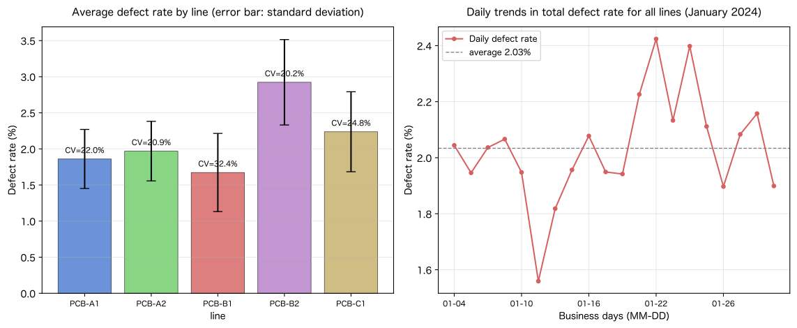
Graph saved: no080_defect_analysis.svg

Reading the results

• df.describe() allows you to check 100 rows x 8 columns of data at once. Maximum value, minimum value, and standard deviation of the number of defects can be instantly grasped.
• Coefficient of variation (CV) shows the following:
  • PCB-B2 (Substrate B-High Density): Maximum CV → Unstable quality, top priority candidate for process improvement
  • PCB-A1 (Substrate A-Small): Minimum CV → Stable process, best practice reference line
• From the daily defect rate trend graph, you can check whether there are any days with a high defect rate on a particular business day.
  If there is a high day, it will be an opportunity to investigate machines, workers, material lots, etc. on that day.

---

Practical implications seen through target exerciseing

Through the introduction to Polars in Nos. 071-080, you will get the following suggestions for manufacturing data analysis.

1. Polars is suitable for large-scale data in the manufacturing industry

When handling monthly/yearly production results (tens of thousands to hundreds of thousands of lines), Polars is superior to pandas in both processing speed and memory efficiency.
It is worth considering introducing Polars as an initial investment for DX promotion.

2. Make the 5 steps of checking data quality a habit

After loading the CSV, be sure to check the following in the following order:

Step	Operation	Check Points
① Check the shape	df.shape	Does it match the expected number of rows and columns?
② Check the beginning and end	df.head() / df.tail()	Are there any extra lines or duplicate headers?
③ Check the column name	df.columns / df.schema	Is the column name correct and correct?
④ Type confirmation	df.dtypes	Is the date of type Date? Is the number Int/Float?
⑤ Check statistics	df.describe()	Are the maximum, minimum, and standard deviation appropriate for business purposes?

3. Line stability can be quickly evaluated using the coefficient of variation (CV)

By calculating the coefficient of variation (CV) from the standard deviation and mean of describe(), Which lines are unstable and need improvement can be prioritized quantitatively.

4. Large-scale data can be processed efficiently in Lazy mode (next step)

This chapter dealt with Eager mode (pl.read_csv), but For millions of rows, the lazy mode of pl.scan_csv → .filter() → .collect() is effective.
Memory shortages can be prevented because only the rows and columns that need to be processed are stored in memory.

What you need to implement in practice

Checklist for full-scale implementation of Polars at the manufacturing site

1. Environmental improvement

• Installed in production environment with pip install polars
• Fixed version to requirements.txt (Example: polars>=1.0,<2.0)
• Decide on coexistence policy with existing pandas code (phased migration or complete replacement)

2. Data pipeline design

• Check the CSV character code, delimiter, and date format and set the read_csv option.
• Check the missing value expression ("NULL", "-", empty string) and specify null_values
• scan_csv → Lazy mode is adopted for large-scale CSV (more than 100,000 lines)

3. Integration into quality management

• Incorporate assert df.shape[0] == Expected number of rows into automatic check after data loading
• Create a type check function and run it every month when CSV is loaded.
• Set the coefficient of variation (CV) threshold and automatically alert when the line is exceeded.

4. Deployment to the team

• Share the basic operations of Polars (contents of this chapter) in a team study session.
• Created a migration guide for pandas users (major operations correspondence table)

Summary

In this chapter (Nos. 071 to 080), you learned the basic operations of Polars using production data from an electronic parts manufacturing factory as the subject matter.

No.	What I learned	Application in the manufacturing industry
071	Role of Polars	Understanding the difference from pandas and deciding whether to apply it to large-scale data
072	Import and confirmation	Importance of recording the execution environment and fixing the version
073	Series creation	Single-column data management such as number of defects and operation rate
074	Creating a DataFrame	Building a production results table from a dictionary
075	CSV loading	Type-safe loading of monthly production results CSV
076	head / tail	Visual confirmation immediately after loading
077	shape	Detect missing days and extra rows by number of rows and columns
078	columns / schema	Batch confirmation and normalization of column names and types
079	dtypes	Correct confirmation of date, number, and string types
080	describe	Evaluate line stability using basic statistics and coefficient of variation

Next chapter (No.081-090) In the next chapter, we will discuss data processing using Polars. (filter, column addition, missing processing, sorting).

Consultation for corporations

For information on promoting DX in the manufacturing industry, building data analysis infrastructure, and in-house Python training, please contact: Please feel free to contact the Surikobo.

📩 Contact: surikobo.co.jp/contact Please feel free to contact us first.

---

*This article is part of the “100 Exercises on Introduction to Python for Data Analysis” series. * *Please check the table of contents for the entire series from here. *