Turning vague consultations about production planning into decision-making models

Basics of Mathematical Modeling Learned at a Precision Parts Factory No.001–No.010

About the 100-Exercise Mathematical Modeling

This article is Mathematical modeling100The Exercise No.1Return. This 100-step approach aims to gradually develop the ability to transform ambiguous on-site issues into mathematical questions, using data, formulas, simulations, and optimization to make explainable decisions.

The entire structure consists of the following 10 chapters.

chapter	No.	Main Themes
Chapter 1	001〜010	Basics of Mathematical Modeling
Chapter 2	011〜020	Expressing data with formulas
Chapter 3	021〜030	Modeling business KPIs
Chapter 4	031〜040	Modeling Demand and Sales
Chapter 5	041〜050	Modeling Inventory and Production
Chapter 6	051〜060	Modeling queues and congestion
Chapter 7	061〜070	Modeling Uncertainty and Risk
Chapter 8	071〜080	State transition model
Chapter 9	081〜090	Modeling for Optimization
Chapter 10	091〜100	Simulation and Decision-Making

This time, we will cover the foundation No.001 to 010. Using the production planning of a precision parts factory as a subject, we transform on-site consultations into mathematical questions, organizing variables, parameters, states, assumptions, units, granularity, constraints, and objective functions to continuously verify the validity of the model.

Before using advanced optimization methods, it is necessary for stakeholders to be able to explain “What do you want to decide?” “What do you think fixedly?” “Which conditions do you follow?” in the same language. Creating fictitious data in Python and connecting mathematical modeling to manufacturing decision-making through tables, graphs, and simple simulations.

[!NOTE] This material is a notebook previously used by Surikoubo (or personally by the representative, Kazuyama), and has been reconstructed, edited, and published with the company’s permission. All data listed is fictional and has no relation whatsoever to real companies, factories, or figures.

Introduction: Practical Challenges in Manufacturing Covered in This Article

At a fictional precision parts factory, the sales department asked us, “Demand will increase next month, so please create a plan to avoid stockouts while not overstocking inventory.” Production management includes records of planned quantities, actual good products, demand, equipment downtime, defect counts, and end-of-period inventory.

However, this request alone cannot be used for calculations. Does “avoiding out-of-stock” mean zero out-of-stock, or is a certain level of service sufficient? How many pieces should be allowed to “not overstock”? Increasing production also includes limits on equipment time, work hours, and materials.

This time, the goal is not to give the only correct answer. It’s about wearing The basic operation of translating field language into verifiable and updatable decision-making models.

Common situations on site

• Demand forecasting, production planning, equipment performance, and quality performance are managed in separate Excel formats
• Qualitative criteria remain for decisions such as “having some leeway” and “minimizing as much as possible.”
• Daily, weekly, and monthly figures are mixed, and even for the same KPI, definitions differ by department.
• Plan with average capacity alone, overlooking valleys caused by daily stops and variety switching.
• Even if you can produce estimated results, you can’t explain which assumptions actually worked for those results.

Mathematical models are not precise models that perfectly replicate the site. It is a tool that retains only the structure necessary for decision-making and clearly indicates the relationship between input and decision results.

Why is this issue so difficult to judge?

In production planning, multiple indicators move simultaneously. Increasing production volume can reduce shortages, but it may also lead to higher overtime costs, work-in-progress inventory, and finished goods inventory. Equipment downtime and defect rates fluctuate daily, so average values alone cannot express the risk of busy periods.

Also, confusing the following three types can make discussions unstable.

1. Facts: Observed values such as past good product count, downtime, and demand
2. assumption: Maintaining yields similar in the future, excluding express orders from regular demand, and so on.
3. Decision-making: Changeable values such as production volume by product, overtime hours, and inventory targets

In mathematical modeling, these are separated, and the units, aggregation granularity, constraints, and evaluation axes are aligned before calculation.

Overview of Exercise covered this time

No.	Theme	Questions in Production Management
001	What is mathematical modeling?	How much can a part of the site be represented by a mathematical formula?
002	Turning business challenges into mathematical questions	How to measure ‘wanting to avoid stockouts’
003	Variables, parameters, and constants	What values should be changed, estimated, or fixed?
004	Input, Output, and Status	How inventory is carried over day by day
005	clarify assumptions	Will the conclusion change depending on how you set stops and yields?
006	Unit, scale, granularity	How to align seconds, hours, individuals, daily and weekly
007	Determining the model’s granularity	How far to track shortages that cannot be seen by monthly averages
008	Organize constraints	Within the limits of equipment, work, and materials,
009	Understanding the objective function	How to Classify Profit, Out-of-Stock, and Inventory as a Single Evaluation Value
010	Validate	Is it accurate enough to use historical data?

No.001 to 010 are not isolated tricks but a series of Setting Challenges → formalization → Reception → verification.

Preparing the Python environment

No external data is used. Fix random numbers in NumPy to generate fictional data, aggregate them with pandas, and visualize them with matplotlib. Graphs are displayed in SVG format to make them easy to read even after Markdown conversion.

%matplotlib inline
%config InlineBackend.figure_format = 'svg'

import platform
import sys

import matplotlib
import matplotlib.pyplot as plt
import numpy as np
import pandas as pd
from IPython.display import display

SEED = 42
rng = np.random.default_rng(SEED)

plt.rcParams["font.family"] = "Hiragino Sans"
plt.rcParams["axes.unicode_minus"] = False
plt.rcParams["figure.figsize"] = (9, 4.8)

print(f"Python     : {sys.version.split()[0]}")
print(f"NumPy      : {np.__version__}")
print(f"pandas     : {pd.__version__}")
print(f"matplotlib : {matplotlib.__version__}")
print(f"platform   : {platform.platform()}")
print(f"random seed: {SEED}")

Python     : 3.13.1
NumPy      : 2.5.1
pandas     : 3.0.3
matplotlib : 3.11.0
platform   : macOS-26.3-arm64-arm-64bit-Mach-O
random seed: 42

Creation of Fictional Data

The target is a fictional factory that manufactures precision pump components. There are three types of products: A, B, and C, with a period of 8 weeks (56 days) starting from April 1, 2025. Each line records “one product per day×

• planned_units: Planned quantity for the day
• demand_units: Demand quantity on the day
• downtime_min: Equipment downtime (minutes)
• defect_rate: Performance Defect Rate
• good_units: Number of good products produced
• ending_inventory: End-of-period inventory after demand allocation

It includes demand schedule, equipment downtime, yield, and capability differences by product. All are imaginary values, and random seed numbers are fixed at 42.

dates = pd.date_range("2025-04-01", periods=56, freq="D")
products = pd.DataFrame({
    "product": ["A", "B", "C"],
    "daily_capacity": [520, 430, 340],
    "standard_defect_rate": [0.018, 0.025, 0.032],
    "cycle_time_sec": [48, 62, 78],
    "material_kg_per_unit": [0.42, 0.55, 0.68],
    "unit_margin_yen": [850, 1100, 1450],
})

rows = []
for day_no, date in enumerate(dates):
    weekday_factor = 0.88 if date.dayofweek >= 5 else 1.04
    trend = 1 + 0.0018 * day_no
    for spec in products.itertuples(index=False):
        demand = max(0, rng.normal(spec.daily_capacity * 0.82 * weekday_factor * trend, 28))
        planned = max(0, rng.normal(spec.daily_capacity * 0.86, 18))
        downtime = np.clip(rng.gamma(shape=1.8, scale=16), 0, 150)
        defect_rate = np.clip(rng.normal(spec.standard_defect_rate, 0.006), 0.004, 0.07)
        available_ratio = max(0, 1 - downtime / (16 * 60))
        produced = min(planned, spec.daily_capacity * available_ratio)
        good_units = np.floor(produced * (1 - defect_rate))
        rows.append({
            "date": date,
            "product": spec.product,
            "planned_units": int(round(planned)),
            "demand_units": int(round(demand)),
            "downtime_min": round(float(downtime), 1),
            "defect_rate": float(defect_rate),
            "good_units": int(good_units),
        })

production = pd.DataFrame(rows).merge(products, on="product", how="left")
production["week"] = ((production["date"] - production["date"].min()).dt.days // 7) + 1

inventory = {"A": 650, "B": 520, "C": 420}
ending_inventory, shortage_units = [], []
for row in production.itertuples(index=False):
    available = inventory[row.product] + row.good_units
    shipped = min(available, row.demand_units)
    shortage = row.demand_units - shipped
    inventory[row.product] = available - shipped
    ending_inventory.append(inventory[row.product])
    shortage_units.append(shortage)

production["ending_inventory"] = ending_inventory
production["shortage_units"] = shortage_units

print(f"Number of records: {len(production):,} Walk ({production['date'].nunique()}days × {production['product'].nunique()}Products)")
display(production.head(9).style.format({"defect_rate": "{:.2%}"}))

Number of records: 168 lines (56 days, × 3 products)

	date	product	planned_units	demand_units	downtime_min	defect_rate	good_units	daily_capacity	standard_defect_rate	cycle_time_sec	material_kg_per_unit	unit_margin_yen	week	ending_inventory	shortage_units
0	2025-04-01 00:00:00	A	428	452	41.200000	0.63%	425	520	0.018000	48	0.420000	850	1	623	0
1	2025-04-01 00:00:00	B	372	330	17.900000	1.99%	364	430	0.025000	62	0.550000	1100	1	554	0
2	2025-04-01 00:00:00	C	306	315	24.800000	3.48%	295	340	0.032000	78	0.680000	1450	1	400	0
3	2025-04-02 00:00:00	A	454	420	9.400000	1.77%	445	520	0.018000	48	0.420000	850	1	648	0
4	2025-04-02 00:00:00	B	358	362	56.000000	2.24%	349	430	0.025000	62	0.550000	1100	1	541	0
5	2025-04-02 00:00:00	C	302	281	31.300000	3.46%	291	340	0.032000	78	0.680000	1450	1	410	0
6	2025-04-03 00:00:00	A	440	505	14.900000	2.17%	430	520	0.018000	48	0.420000	850	1	573	0
7	2025-04-03 00:00:00	B	368	400	10.700000	2.89%	357	430	0.025000	62	0.550000	1100	1	498	0
8	2025-04-03 00:00:00	C	302	312	12.800000	3.27%	292	340	0.032000	78	0.680000	1450	1	390	0

overview = production.groupby("product", as_index=False).agg(
    planned_number=("planned_units", "sum"),
    good_quantity=("good_units", "sum"),
    demand=("demand_units", "sum"),
    number_of_items_out_of_stock=("shortage_units", "sum"),
    average_defect_rate=("defect_rate", "mean"),
    stop_time_minutes=("downtime_min", "sum"),
    final_stock=("ending_inventory", "last"),
)
display(overview.style.format({"average_defect_rate": "{:.2%}", "stop_time_minutes": "{:,.1f}"}))
print(
    f"Total for the entire period | good product {production['good_units'].sum():,}units / "
    f"need {production['demand_units'].sum():,}units / missing item {production['shortage_units'].sum():,}units"
)

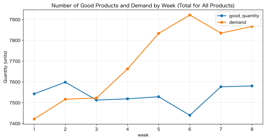
weekly = production.groupby("week", as_index=False).agg(
    good_quantity=("good_units", "sum"), demand=("demand_units", "sum"), number_of_items_out_of_stock=("shortage_units", "sum")
)
ax = weekly.plot(x="week", y=["good_quantity", "demand"], marker="o", linewidth=2)
ax.set_title("Number of Good Products and Demand by Week (Total for All Products)")
ax.set_xlabel("week")
ax.set_ylabel("Quantity (units)")
ax.grid(True, alpha=0.3)
plt.tight_layout()
plt.show()

	product	planned_number	good_quantity	demand	number_of_items_out_of_stock	average_defect_rate	Stop time_minutes	final_stock
0	A	24805	24330	24823	0	1.71%	1,531.5	157
1	B	20776	20241	20547	0	2.43%	1,427.9	214
2	C	16272	15722	16205	66	3.20%	1,767.8	3

Total for all periods | Good Condition 60,293 units / Needed 61,575 units / Missing 66 units

---

No.001: Understanding What Mathematical Modeling Is

Meaning in Practice

Mathematical modeling is not about reproducing everything on site, but about selecting elements related to judgment and representing them as relationships between quantities. For example, if you consider the number of good products, keep the planned quantity, equipment availability ratio, and yield, and omit worker names and slip numbers if unnecessary for this decision.

Approach to Analysis and Modeling

Place the simplified good quantity model as follows.

$$\widehat{Q}_{d,p}=\min(P_{d,p},\ C_p A_{d,p})\,(1-r_p)$$

• $\widehat{Q}_{d,p}$: Predicted number of good products per day $d$ and product $p$
• $P_{d,p}$: Planned Number
• $C_p$: Daily Capacity
• $A_{d,p}=1-\frac{T_{d,p}}{960}$: Utilization rate for 16 hours (960 minutes)
• $r_p$: Standard Defect Rate

This formula multiplies the standard yield by the lower of the planned number and post-stop capacity. Because we narrow down real-world factors, margins of error remain. Check whether this error is acceptable for decision-making purposes in No.010.

Check with Python

production["modeled_good_units"] = np.floor(
    np.minimum(
        production["planned_units"],
        production["daily_capacity"] * (1 - production["downtime_min"] / 960),
    ) * (1 - production["standard_defect_rate"])
).astype(int)

model_example = production.loc[:8, [
    "date", "product", "planned_units", "downtime_min",
    "good_units", "modeled_good_units"
]].copy()
model_example["error_units"] = model_example["modeled_good_units"] - model_example["good_units"]
display(model_example)

	date	product	planned_units	downtime_min	good_units	modeled_good_units	error_units
0	2025-04-01	A	428	41.2	425	420	-5
1	2025-04-01	B	372	17.9	364	362	-2
2	2025-04-01	C	306	24.8	295	296	1
3	2025-04-02	A	454	9.4	445	445	0
4	2025-04-02	B	358	56.0	349	349	0
5	2025-04-02	C	302	31.3	291	292	1
6	2025-04-03	A	440	14.9	430	432	2
7	2025-04-03	B	368	10.7	357	358	1
8	2025-04-03	C	302	12.8	292	292	0

Reading the results

The forecast values do not exactly match the actual number of good products. This is because only the standard defect rate is used, omitting daily minor stoppages and quality fluctuations. On the other hand, the framework that the number of good products is determined by planned quantity, capacity, stopping capacity, and yield can be explained.

In practice, the required accuracy is determined not only by “precision” but also by Which model should you use for judgment?. The required granularity differs between the model that looks at monthly estimated capacity and the model that determines the order of delivery on the day.

---

No.002: Turning Business Challenges into Mathematical Questions

Meaning in Practice

Simply “wanting to avoid stockouts” is not enough to determine achievement. By defining the target period, target products, demand, and allowable shortage quantities, stakeholders can address the same questions.

Approach to Analysis and Modeling

This time, we will transform the business issue into the following questions.

For each week and each product, can demand be met by starting inventory and forecasted good product count? If you can’t meet the requirements, how many are missing?

If we take the supply-demand difference for weekly $w$ and product $p$ as $G_{w,p}$,

$$G_{w,p}=I_{w,p}^{\mathrm{begin}}+Q_{w,p}-D_{w,p}$$

The shortage is $S_{w,p}=\max(0,-G_{w,p})$. This definition replaces “dangerous” with the KPI of missing quantities.

Check with Python

weekly_product = production.groupby(["week", "product"], as_index=False).agg(
    predicted_good_quantity=("modeled_good_units", "sum"),
    demand=("demand_units", "sum"),
)
weekly_product["Beginning inventory"] = weekly_product["product"].map({"A": 650, "B": 520, "C": 420})
weekly_product.loc[weekly_product["week"] > 1, "Beginning inventory"] = 0
weekly_product["supply-demand gap"] = (
    weekly_product["Beginning inventory"] + weekly_product["predicted_good_quantity"] - weekly_product["demand"]
)
weekly_product["Shortfall Forecast"] = (-weekly_product["supply-demand gap"]).clip(lower=0)

display(weekly_product.pivot(index="week", columns="product", values="supply-demand gap").style
        .format("{:+,.0f}").background_gradient(cmap="RdYlGn", vmin=-250, vmax=250))
print(f"Combinations expected to be insufficient in simple weekly judgment: {(weekly_product['Shortfall Forecast'] > 0).sum()}records / {len(weekly_product)}records")

product	A	B	C
week
1	+677	+540	+483
2	+136	-44	-17
3	+61	+59	-105
4	-98	-97	+53
5	-212	+14	-120
6	-116	-241	-142
7	-183	+6	-99
8	-128	-36	-114

Combinations expected to be insufficient in simple weekly judgment: 15 / 24

Reading the results

Even for the same “shortage concern,” breaking down products and weekly items reveals priorities. Negative weeks are those when, ignoring carryover from the previous week, the simplified judgment exceeded the predicted number of good products.

What is important here is to fix the question before calculating. In actual operations, we add operational rules such as “carrying over year-end inventory to the next week,” “carrying over order backlogs to the next day,” and “adding safety stock to demand.”

---

No.003: Understanding the Differences Between Variables, Parameters, and Constants

Meaning in Practice

If you treat all model values equally, responsibility becomes ambiguous. Production quantity is a value decided in meetings, yield is estimated from actual results, and 1 hour = 60 minutes is a fixed value by definition.

Approach to Analysis and Modeling

Types	Meaning	This time’s example
decision variable	Values chosen by the person in charge	Production Planned Quantity by Product $x_p$
Parameter	Values given from data and estimates	Defect rate $r_p$, $D_p$, capability $C_p$
constant	Values that are fixed by definition	1 hour = 60 minutes, applicable period = 7 days

Even with a simple predicted quantity of good products $Q=x(1-r)$, distinguishing between variable $x$ and parameter $r$ allows you to estimate the effects of “increased production” and “quality improvement” separately.

Check with Python

base_plan = 3_000  # Decision variable x
defect_candidates = [0.015, 0.025, 0.035]  # Assumptions for parameter r
plan_candidates = [2_800, 3_000, 3_200]

sensitivity = pd.DataFrame([
    {"planned_number_x": x, "defect_rate_r": r, "predicted_good_quantity_Q": round(x * (1 - r))}
    for x in plan_candidates for r in defect_candidates
])
pivot = sensitivity.pivot(index="planned_number_x", columns="defect_rate_r", values="predicted_good_quantity_Q")
pivot.columns = [f"defect rate {r:.1%}" for r in pivot.columns]
display(pivot)

	defect_rate 1.5%	defect_rate 2.5%	defect_rate 3.5%
planned_number_x
2800	2758	2730	2702
3000	2955	2925	2895
3200	3152	3120	3088

Reading the results

Even with the same plan of 3,000 units, if the defect rate estimate changes from 1.5% to 3.5%, the number of good products changes. Conversely, fixing the defect rate allows you to compare the effectiveness of increasing the planned quantity.

In practice, approval permissions are assigned to decision variables, and parameters are assigned sources and update frequency. For example, if you decide that “the standard defect rate is updated monthly by quality control” or “production plans are determined weekly by production management,” the model becomes less personalized and less personalized.

---

No.004: Organizing Input, Output, and State

Meaning in Practice

Inventory and work-in-progress results carry over to the next day. Instead of independent daily aggregation, we need a model with a state.

Approach to Analysis and Modeling

Update the inventory status of product $p$ using the following formula.

$$I_{d,p}^{\mathrm{end}}=\max\left(0, I_{d,p}^{\mathrm{begin}}+Q_{d,p}-D_{d,p}\right)$$ $$S_{d,p}=\max\left(0, D_{d,p}-I_{d,p}^{\mathrm{begin}}-Q_{d,p}\right)$$

• Input: Number of good goods on the day $Q$, demand $D$
• Condition: Beginning and ending inventory $I$
• exert effort: Shipped quantity, out-of-stock quantity $S$

This time, as a lost order, out-of-stock items are not carried over to the next day. If the task is carried over as a backlog, add the backorder status.

Check with Python

sample_a = production.query("product == 'A'").head(14).copy()
state = 650
states = []
for row in sample_a.itertuples(index=False):
    begin = state
    available = begin + row.good_units
    shortage = max(0, row.demand_units - available)
    state = max(0, available - row.demand_units)
    states.append((begin, row.good_units, row.demand_units, state, shortage))

state_table = pd.DataFrame(states, columns=["Beginning inventory", "good_quantity", "demand", "ending inventory", "number_of_items_out_of_stock"])
state_table.insert(0, "Date", sample_a["date"].dt.strftime("%m-%d").to_numpy())
display(state_table)

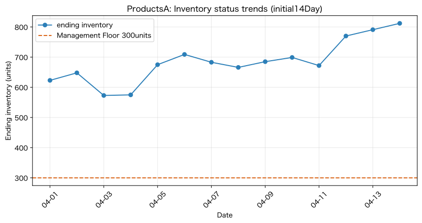
ax = state_table.plot(x="Date", y="ending inventory", marker="o", color="#2c7fb8", legend=False)
ax.axhline(300, color="#d95f0e", linestyle="--", label="Management Floor 300units")
ax.set_title("ProductsA: Inventory status trends (initial14Day)")
ax.set_xlabel("Date")
ax.set_ylabel("Ending inventory (units)")
ax.grid(True, alpha=0.3)
ax.legend()
plt.xticks(rotation=45)
plt.tight_layout()
plt.show()

	Date	Beginning inventory	good_quantity	demand	ending inventory	number_of_items_out_of_stock
0	04-01	650	425	452	623	0
1	04-02	623	445	420	648	0
2	04-03	648	430	505	573	0
3	04-04	573	454	452	575	0
4	04-05	575	431	331	675	0
5	04-06	675	432	398	709	0
6	04-07	709	441	467	683	0
7	04-08	683	426	443	666	0
8	04-09	666	440	421	685	0
9	04-10	685	436	422	699	0
10	04-11	699	420	447	672	0
11	04-12	672	455	357	770	0
12	04-13	770	441	420	791	0
13	04-14	791	450	429	812	0

Reading the results

Inventory depends not only on the quantity and demand of good products on that day but also on the previous day’s year-end stock. Therefore, the day demand exceeds production does not necessarily mean the out-of-stock date is immediately triggered. On the other hand, if inventory continues to decrease, even small increases in demand later can lead to shortages.

By clearly stating the status, it connects to operational rules such as “when to make replenishment decisions” and “how many management floors to set.”

---

No.005: Clarifying the Assumptions Needed for Modeling

Meaning in Practice

Future downtime and defect rates have not been finalized. Showing multiple scenarios that alter assumptions better helps decision-makers better understand risk than a single forecast that hides assumptions.

Approach to Analysis and Modeling

For the next week plan for Product B, let’s compare the following assumptions.

• Optimism: 10-minute downtime per day, defect rate 2.0%
• Standard: Downtime 30 minutes/day, defect rate 2.5%
• Caution: Downtime 75 minutes/day, defect rate 4.0%

For each scenario, calculate $Q=\min(P,CA)(1-r)$. Assuming demand is 3,000 units and the beginning inventory is 200 units. Assumptions are not predictions but inputs to gauge the breadth of judgment.

Check with Python

scenario = pd.DataFrame({
    "Scenario": ["optimism", "standard", "cautious"],
    "Stop time_day by day": [10, 30, 75],
    "defect_rate": [0.020, 0.025, 0.040],
})
days = 7
daily_plan_b = 430
demand_b = 3_000
begin_inventory_b = 200
scenario["predicted_good_quantity"] = np.floor(
    np.minimum(daily_plan_b, 430 * (1 - scenario["Stop time_day by day"] / 960))
    * (1 - scenario["defect_rate"]) * days
).astype(int)
scenario["surplus capacity"] = begin_inventory_b + scenario["predicted_good_quantity"] - demand_b
display(scenario.style.format({"defect_rate": "{:.1%}", "surplus capacity": "{:+,}"}))

	Scenario	Stop time_day by day	defect_rate	predicted_good_quantity	surplus capacity
0	optimism	10	2.0%	2919	+119
1	standard	30	2.5%	2843	+43
2	cautious	75	4.0%	2663	-137

Reading the results

Even with the same planned quantity, supply and demand capacity varies depending on assumptions of downtime and defect rates. Even if the base scenario alone provides some margin, if the cautionary scenario is insufficient, it provides grounds to consider adjustments to maintenance schedules, support personnel, outsourcing, and advance inventory.

In practice, the list of assumptions includes the basis, responsible person, update date, and validity period. This model includes operations where “recalculation occurs when assumptions are wrong.”

---

No.006: Align Units, Scales, and Granularity

Meaning in Practice

In manufacturing data, cycle times may be recorded in seconds per piece, stoppage times in minutes, operating slots in hours, and materials in kilograms. If you add, subtract, multiply, and divide without matching the units, the calculation will lose its meaning even if it works.

Approach to Analysis and Modeling

Production time is converted to time using the following formula.

$$H_p=\frac{x_p\,t_p}{3600}$$

$x_p$ is the number of pieces produced, $t_p$ is per second, and $H_p$ is time. The denominator of 3,600 is a constant that converts seconds into time. Also, when comparing, the period granularity is aligned for daily or weekly intervals.

Check with Python

unit_check = products[["product", "cycle_time_sec", "material_kg_per_unit"]].copy()
unit_check["planned quantity_units"] = [3_200, 2_700, 2_100]
unit_check["Required equipment time_hours"] = (
    unit_check["planned quantity_units"] * unit_check["cycle_time_sec"] / 3_600
)
unit_check["Required Materials_kg"] = (
    unit_check["planned quantity_units"] * unit_check["material_kg_per_unit"]
)
display(unit_check.style.format({"Required equipment time_hours": "{:,.1f}", "Required Materials_kg": "{:,.1f}"}))

daily_total = production.groupby("date", as_index=False)[["good_units", "demand_units"]].sum()
weekly_total = production.groupby("week", as_index=False)[["good_units", "demand_units"]].sum()
print(f"Average daily demand: {daily_total['demand_units'].mean():,.1f} units/days")
print(f"Weekly average demand: {weekly_total['demand_units'].mean():,.1f} units/week")
print(f"daily average × 7: {daily_total['demand_units'].mean() * 7:,.1f} units/week")

	product	cycle_time_sec	material_kg_per_unit	planned quantity_units	Required equipment time_hours	Required Materials_kg
0	A	48	0.420000	3200	42.7	1,344.0
1	B	62	0.550000	2700	46.5	1,485.0
2	C	78	0.680000	2100	45.5	1,428.0

Average daily requirement: 1,099.6 units/day
Average weekly required: 7,696.9 days/week
Daily average × 7: 7,696.9 units/week

Reading the results

The value obtained by multiplying the number of units per second is in seconds, so you need to divide by 3,600 to compare it to the equipment slot in the hour unit. Similarly, multiplying the number of pieces by kg gives the required material in kilograms.

In the data dictionary, not only column names but also definitions such as unit, time granularity, tax included and excluded, good quality and gross production are included. Including units in the list is also a practical way to reduce accidents.

---

No.007: Determining the Model Granularity

Meaning in Practice

Even if supply and demand match week-over-week, daily shortages can occur if demand concentrates in the first half of the week. The finer the model, the more information can be preserved, but it also increases the burden of data preparation, calculation, and explanation.

Approach to Analysis and Modeling

Granularity is not “finer is better,” but rather aligns with the decision cycle and risk.

• Monthly: Review of medium-term capabilities and budget
• Weekly: Adjustments to production volume, personnel, and materials
• Daily: Inventory and Delivery Schedule Management
• By time of day: deployment order, planning, bottleneck management

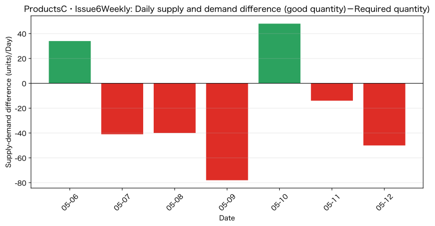
Here, for product C in week 6, we compare the daily shortage and the weekly total supply-demand difference.

Check with Python

granularity = production.query("week == 6 and product == 'C'").copy()
granularity["daily supply and demand difference"] = granularity["good_units"] - granularity["demand_units"]
granularity_view = granularity[["date", "good_units", "demand_units", "daily supply and demand difference"]]
display(granularity_view.style.format({"daily supply and demand difference": "{:+,}"}))

weekly_gap = granularity["daily supply and demand difference"].sum()
daily_negative = (-granularity["daily supply and demand difference"]).clip(lower=0).sum()
print(f"Weekly total supply-demand difference         : {weekly_gap:+,} units")
print(f"Total for the daily shortage only : {daily_negative:,} units")
print(f"Number of Rows to Compare (Daily/Weekly): {len(granularity)} rows / 1 rows")

fig, ax = plt.subplots()
colors = np.where(granularity["daily supply and demand difference"] >= 0, "#2ca25f", "#de2d26")
ax.bar(granularity["date"].dt.strftime("%m-%d"), granularity["daily supply and demand difference"], color=colors)
ax.axhline(0, color="black", linewidth=0.8)
ax.set_title("ProductsC・Issue6Weekly: Daily supply and demand difference (good quantity)－Required quantity)")
ax.set_xlabel("Date")
ax.set_ylabel("Supply-demand difference (units)/Day)")
ax.grid(True, axis="y", alpha=0.3)
plt.xticks(rotation=45)
plt.tight_layout()
plt.show()

	date	good_units	demand_units	daily supply and demand difference
107	2025-05-06 00:00:00	298	264	+34
110	2025-05-07 00:00:00	286	327	-41
113	2025-05-08 00:00:00	294	334	-40
116	2025-05-09 00:00:00	242	320	-78
119	2025-05-10 00:00:00	275	227	+48
122	2025-05-11 00:00:00	264	278	-14
125	2025-05-12 00:00:00	275	325	-50

Weekly total supply-demand difference: -141 units
Total daily shortage only for the side: 223
Number of Rows Compared (Daily/Weekly): 7 lines / 1 row

Reading the results

The weekly total offsets the gains and losses within the week. If the beginning inventory is sufficient, offsetting is not a problem, but if inventory is low, same-day delivery is required, or early production cannot be done, daily shortages become important.

The required granularity is determined by business rules. This time, a realistic two-stage design is to create rough weekly capacity plans and dig into only products with high shortage risk daily.

---

No.008: Organizing Constraints

Meaning in Practice

If the idea of “making a lot” exceeds equipment time, work time, materials, and storage space, it cannot be implemented. Constraints are the conditions that divide candidate proposals into feasible and impossible.

Approach to Analysis and Modeling

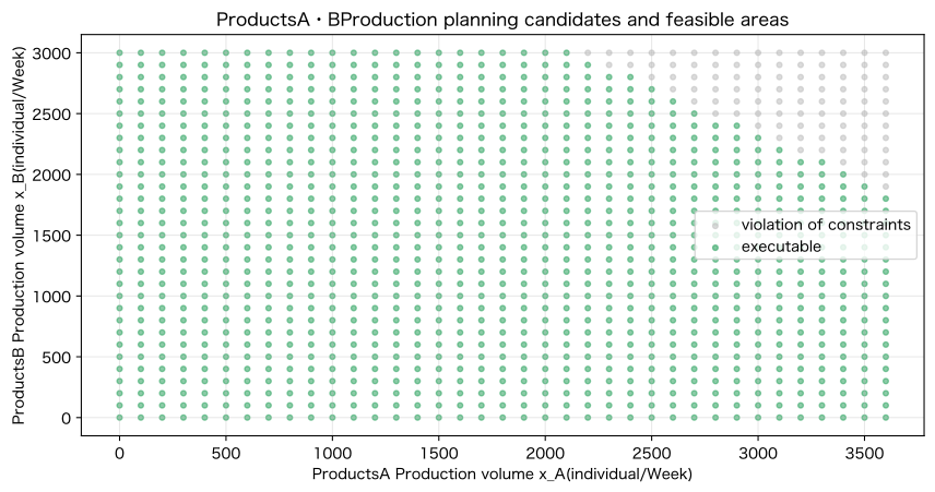
Let the production volume of products A and B for the following week be $x_A,x_B$. For simplicity, the following constraints are placed.

$$\frac{48x_A+62x_B}{3600}\leq 86 \quad \text{(Equipment Time)}$$ $$0.030x_A+0.040x_B\leq 190\quad\text{(Operation time)}$$ $$0.42x_A+0.55x_B\leq 2550 \quad \text{(material)}$$

Furthermore, let’s say $0\leq x_A\leq 3600$, $0\leq x_B\leq 3000$. Here, you search for all candidates in increments of 100 and confirm plans that meet the constraints.

Check with Python

plans = []
for x_a in range(0, 3_601, 100):
    for x_b in range(0, 3_001, 100):
        machine_h = (48 * x_a + 62 * x_b) / 3_600
        labor_h = 0.030 * x_a + 0.040 * x_b
        material_kg = 0.42 * x_a + 0.55 * x_b
        feasible = machine_h <= 86 and labor_h <= 190 and material_kg <= 2_550
        plans.append((x_a, x_b, machine_h, labor_h, material_kg, feasible))

plans = pd.DataFrame(plans, columns=[
    "x_A", "x_B", "Facility Hours", "Working hours", "Ingredientskg", "executable"
])
print(f"Number of candidates: {len(plans):,}records / executable: {plans['executable'].sum():,}records")
display(plans.query("`executable`").sort_values(["x_A", "x_B"], ascending=False).head(10)
        .style.format({"Facility Hours": "{:.1f}", "Working hours": "{:.1f}", "Ingredientskg": "{:.1f}"}))

fig, ax = plt.subplots()
for feasible, group in plans.groupby("executable"):
    ax.scatter(group["x_A"], group["x_B"], s=13, alpha=0.55,
               label="executable" if feasible else "violation of constraints",
               color="#2ca25f" if feasible else "#bdbdbd")
ax.set_title("ProductsA・BProduction planning candidates and feasible areas")
ax.set_xlabel("ProductsA Production volume x_A(individual/Week)")
ax.set_ylabel("ProductsB Production volume x_B(individual/Week)")
ax.grid(True, alpha=0.3)
ax.legend()
plt.tight_layout()
plt.show()

Number of candidates: 1,147 / Feasible: 1,052

	x_A	x_B	Facility Hours	Working hours	Ingredientskg	executable
1134	3600	1800	79.0	180.0	2502.0	True
1133	3600	1700	77.3	176.0	2447.0	True
1132	3600	1600	75.6	172.0	2392.0	True
1131	3600	1500	73.8	168.0	2337.0	True
1130	3600	1400	72.1	164.0	2282.0	True
1129	3600	1300	70.4	160.0	2227.0	True
1128	3600	1200	68.7	156.0	2172.0	True
1127	3600	1100	66.9	152.0	2117.0	True
1126	3600	1000	65.2	148.0	2062.0	True
1125	3600	900	63.5	144.0	2007.0	True

Reading the results

Gray candidates violate at least one constraint. The green range indicates a feasible plan under current conditions. Visualizing constraints makes it easier to discuss whether to increase equipment, whether to increase material procurement, and whether work improvements are effective.

For production models, constraint candidates include the number of setup cycles, minimum lot size, integer quantity, shared facilities with product C, and maintenance time. Don’t include everything from the start; instead, add the conditions that determine the feasibility of the plan.

---

No.009: Understanding the Concept of Objective Functions

Meaning in Practice

There is not always just one viable plan. The objective function serves as the standard for comparing which candidate is desirable. This may include not only profit maximization but also out-of-stock items, overtime, inventory, and delivery delays.

Approach to Analysis and Modeling

Set demand to $D_A=3,100$, $D_B=2,500$, initial inventory to 100 units each, and set the valuation profit as follows.

$$Z=\sum_p m_p\min(D_p,I_p+x_p)-c_s S_p-c_h E_p-c_o O$$

• $m_p$: Marginal profit per unit sold
• $S_p$: Number of items out, $c_s$: Out-of-stock penalty
• $E_p$: Ending Inventory, $c_h$: Inventory Holding Cost
• $O$: Facility hours exceeding 80 hours, $c_o$: Additional operating costs

Penalties are not a “true loss” but a quantified management priority. A sensitivity analysis with different values is required.

Check with Python

demand = {"A": 3_100, "B": 2_500}
initial_inventory = {"A": 100, "B": 100}
margin = {"A": 850, "B": 1_100}
shortage_penalty = 1_800
holding_cost = 90
overtime_cost_per_h = 18_000

candidate = plans.query("`executable`").copy()
for p in ["A", "B"]:
    available = candidate[f"x_{p}"] + initial_inventory[p]
    candidate[f"Sales_{p}"] = np.minimum(available, demand[p])
    candidate[f"missing item_{p}"] = np.maximum(0, demand[p] - available)
    candidate[f"Inventory_{p}"] = np.maximum(0, available - demand[p])

candidate["Additional operating hours"] = np.maximum(0, candidate["Facility Hours"] - 80)
candidate["valuation profit"] = (
    candidate["sales_A"] * margin["A"] + candidate["sales_B"] * margin["B"]
    - (candidate["missing_item_A"] + candidate["missing_item_B"]) * shortage_penalty
    - (candidate["Inventory_A"] + candidate["Inventory_B"]) * holding_cost
    - candidate["Additional operating hours"] * overtime_cost_per_h
)

best_plans = candidate.nlargest(8, "valuation profit")[[
    "x_A", "x_B", "Facility Hours", "Working hours", "missing_item_A", "missing_item_B",
    "Inventory_A", "Inventory_B", "valuation profit"
]]
display(best_plans.style.format({
    "Facility Hours": "{:.1f}", "Working hours": "{:.1f}", "valuation profit": "¥{:,.0f}"
}))
best = best_plans.iloc[0]
print(
    f"Recommended Candidates: A={int(best['x_A']):,}Individual,B={int(best['x_B']):,}Individual,"
    f"valuation profit=¥{best['valuation profit']:,.0f}"
)

	x_A	x_B	Facility Hours	Working hours	missing_item_A	missing_item_B	Inventory_A	Inventory_B	valuation profit
923	2900	2400	80.0	183.0	100	0	0	0	¥5,120,000
953	3000	2300	79.6	182.0	0	100	0	0	¥5,095,000
892	2800	2400	78.7	180.0	200	0	0	0	¥4,855,000
922	2900	2300	78.3	179.0	100	100	0	0	¥4,830,000
952	3000	2200	77.9	178.0	0	200	0	0	¥4,805,000
983	3100	2200	79.2	181.0	0	200	100	0	¥4,796,000
861	2700	2400	77.3	177.0	300	0	0	0	¥4,590,000
862	2700	2500	79.1	181.0	300	0	0	100	¥4,581,000

Recommended candidates: A = 2,900 units, B = 2,400 units, Evaluation profit = ¥5,120,000

Reading the results

By ranking actionable candidates with the objective function, you can compare recommended plans with proximity candidates. Rather than just presenting the top spot, showing the differences between the second and third place, the breakdown of out-of-stock, and the margin of constraints makes it easier for the field to decide whether to accept the position.

The objective function is where management policies are converted into formulas. Consensus is necessary, such as making out-of-stock for key customers heavier than general inventory, or making overtime limits rather than penalties.

---

No.010: Organize the perspectives to verify the validity of the model

Meaning in Practice

Even if the formula works correctly, it does not necessarily mean it can be used for on-site judgment. Forecast errors are measured using historical data to identify biases and significant deviations by product. Not only average error, but also the direction of over-prediction and under-forecasting is important.

Approach to Analysis and Modeling

Compare the predicted number of good products for No.001 with the actual results and check the following.

$$\mathrm{MAE}=\frac{1}{n}\sum_{i=1}^{n}|\widehat{Q}_i-Q_i|$$ $$\mathrm{MAPE}=\frac{100}{n}\sum_{i=1}^{n}\left|\frac{\widehat{Q}_i-Q_i}{Q_i}\right|$$ $$\mathrm{Bias}=\frac{1}{n}\sum_{i=1}^{n}(\widehat{Q}_i-Q_i)$$

MAE indicates the average quantity error, MAPE is the margin of error relative to size, and Bias indicates the direction of over-or under-forecasting. Furthermore, input definitions, extreme conditions, business rules, and explainability are also subject to validation.

Check with Python

validation = production.copy()
validation["error"] = validation["modeled_good_units"] - validation["good_units"]
validation["abs_error"] = validation["error"].abs()
validation["ape"] = validation["abs_error"] / validation["good_units"].clip(lower=1)

metrics = validation.groupby("product", as_index=False).agg(
    number_of_cases=("error", "size"),
    mae=("abs_error", "mean"),
    MAPE=("ape", "mean"),
    bias=("error", "mean"),
    maximum_absolute_error_pieces=("abs_error", "max"),
)
overall = pd.DataFrame({
    "product": ["Overall"],
    "number_of_cases": [len(validation)],
    "mae": [validation["abs_error"].mean()],
    "MAPE": [validation["ape"].mean()],
    "bias": [validation["error"].mean()],
    "maximum_absolute_error_pieces": [validation["abs_error"].max()],
})
metrics_display = pd.concat([metrics, overall], ignore_index=True)
display(metrics_display.style.format({
    "mae": "{:.2f}", "MAPE": "{:.2%}", "bias": "{:+.2f}", "maximum_absolute_error_pieces": "{:.0f}"
}))
print(
    f"overall indicator | MAE={validation['abs_error'].mean():.2f}Individual,"
    f"MAPE={validation['ape'].mean():.2%}、Bias={validation['error'].mean():+.2f}units"
)

fig, axes = plt.subplots(1, 2, figsize=(11, 4.5))
for product, group in validation.groupby("product"):
    axes[0].scatter(group["good_units"], group["modeled_good_units"], s=24, alpha=0.6, label=product)
low = min(validation["good_units"].min(), validation["modeled_good_units"].min())
high = max(validation["good_units"].max(), validation["modeled_good_units"].max())
axes[0].plot([low, high], [low, high], "k--", linewidth=1)
axes[0].set_title("Comparison of Actual Good Units and Model Predictions")
axes[0].set_xlabel("Actual Good Items (units)/Day)")
axes[0].set_ylabel("Predicted Good Quantity (units)/Day)")
axes[0].grid(True, alpha=0.3)
axes[0].legend(title="Products")

axes[1].hist(validation["error"], bins=17, color="#756bb1", edgecolor="white")
axes[1].axvline(0, color="black", linestyle="--", linewidth=1)
axes[1].set_title("Distribution of prediction error (prediction－Track record)")
axes[1].set_xlabel("Error (units)/Day)")
axes[1].set_ylabel("number_of_cases")
axes[1].grid(True, axis="y", alpha=0.3)
plt.tight_layout()
plt.show()

	product	number_of_cases	MAE_units	MAPE	Bias_units	maximum absolute error_units
0	A	56	2.43	0.56%	-0.36	8
1	B	56	1.80	0.49%	-0.23	5
2	C	56	1.14	0.41%	+0.04	4
3	Overall	168	1.79	0.49%	-0.18	8

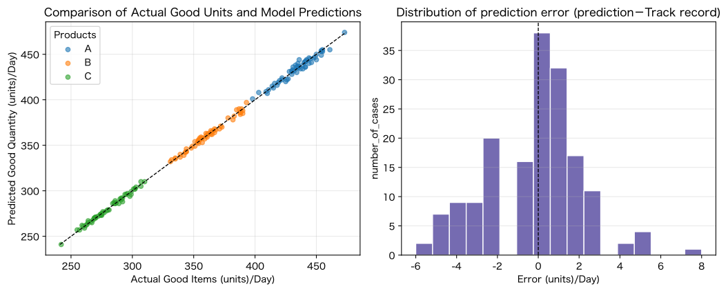
Overall Metrics | MAE = 1.79 points, MAPE = 0.49%, Bias = -0.18 points

Reading the results

The closer the scatter plot is to the 45th parallel, the closer the forecast is to the actual results. If Bias is positive, the average is an overforecast; if negative, it is an underestimate. By generating errors by product, you can identify biases hidden in the overall average.

Since this model does not know the daily actual defect rate before forecasting, it uses standard defect rates. If the error exceeds acceptable limits, options include explanatory variables such as temperature, work group, setup, and material lots. However, the maintenance burden and explanation difficulties caused by adding variables are also evaluated simultaneously.

---

Practical Implications Seen Through Target Exercise

An important insight from these 10 papers is that there is Designing Decisions before algorithm selection.

1. Transform business issues into mathematical questions with targets, durations, KPIs, and acceptable limits.
2. Separate decision variables, estimated parameters, and constants, and determine update responsibilities.
3. The amount carried over from a previous point, such as inventory, is modeled as a state
4. Assume without hiding assumptions, and assess the robustness of conclusions through scenarios of optimism, standards, and caution.
5. Align the units and granularity to select the fineness needed for the decision cycle.
6. Ensuring feasibility with constraints and comparing desirability with objective functions
7. Identify discrepancies, biases, and exceptions against actual performance, and monitor during operation

Even with small models, if assumptions and evaluation axes are shared, meetings can be organized without denying experiential knowledge.

What is necessary for practical implementation

1. Define decision-making and users first

Clarify whether the weekly production meeting will determine the quantity by product or whether the order of shipments will be changed at the daily morning meeting. The decision cycle determines the model’s granularity and update time.

2. Define and Define Data Quality

Define and close the units for planned quantities, actual quantities, good product quantities, demand, shipments, stockouts, and inventory. It is also necessary to handle missing measurements, later corrections, and equipment code changes.

3. Agree on assumptions, constraints, and objective functions among the relevant departments

In production management, manufacturing, quality, maintenance, sales, and accounting, we verify capabilities, defect rates, key customers, overtime costs, and the impact of out-of-stock situations. More important than the formula itself, it is important to agree on the business rules that will be included in it.

4. Start with Parallel Evaluation Alongside Current Judgments

Instead of auto-deciding from the start, compare model proposals with current plans in parallel. Review the days when differences occurred to identify unreflected constraints and exceptions.

5. Create monitoring and update mechanisms

Regularly monitor MAE, Bias, out-of-stock rates, inventory, and the number of plan changes. You also decide on parameter update frequency, conditions for relearning and reestimation, manual operation during failures, and the model manager.

6. Implement small and measure effectiveness through pricing and operational metrics

Starting from one product and one line, we measure reductions in stockouts, overtime, inventory, and shortened planning time. After confirming the effectiveness and maintenance burden, we expand the scope.

Conclusion

In No.001–010, we used fictitious data from precision parts factories to confirm the foundation of mathematical modeling.

• A model is not a copy of reality, but a representation of the structure necessary for decision-making
• Ambiguous issues are transformed into mathematical questions with subjects, durations, and KPIs.
• Distinguish between variables, parameters, constants, input, output, and state
• Specify assumptions, units, and time granularity
• Executability by constraint, desirability by objective function
• Identify discrepancies and biases with past performance and assess the validity of the intended use.

The value of mathematical modeling lies not in using complex formulas, but in making the assumptions of decisions and trade-offs visible.

Consultations for Corporations

At Surikoubo, we support the following themes in manufacturing.

• Model design for production planning, staffing, and equipment allocation
• Managing trade-offs in inventory, out-of-stock, delivery dates, and overtime
• Definition, KPI Design, and Visualization of On-Site Data
• PoC of Mathematical Optimization, Simulation, and Prediction Models
• Real-data-based training for on-site staff and managers
• Establishing a system for decision support based on existing Excel operations

From the stage of “There are challenges but we don’t know what formulas to use,” we can consult on everything from business hearings, data verification, small-scale verification, to practical operational design.

📩 Contact Us: surikobo.co.jp/contact Please feel free to consult us first.