
100 Exercises / column / 100 Exercises in the Line
Learning Manufacturing Quality Forecasting with Python | Introduction to Ridge, Logistic Regression, and Attention
Predict quality risks from processing conditions and determine conditions for improvement
Learning Manufacturing Matrix Analysis with Optimization, Regression, and Attention: 100 Exercises No.051–No.060
In manufacturing sites, factors such as processing speed, feed rate, temperature, vibration, and tool wear all simultaneously affect quality. This article uses a fictional precision parts line as the subject and addresses Predict quality errors, quantify defect risks, stabilize calculations, and narrow down key processes to be checked. from the perspective of a queue.
[!NOTE] This material is a notebook previously used by Surikoubo (or personally by the representative, Kazuyama), and has been reconstructed, edited, and published with the company’s permission.
All data listed is fictional and has no relation whatsoever to real companies, factories, or figures.
Introduction: Practical Challenges in Manufacturing Covered in This Article
In a fictional factory, precision shafts are machined by lots, recording dimensional errors and final inspection pass/fail. Manufacturing engineers aim to predict dimensional errors based on processing conditions and equipment conditions, prioritize lots with a high probability of defects for inspection, and establish a basis for reviewing conditions.
The important thing is not just to create predictive values. It can explain up to Which calculation method is stable, can it capture nonlinear quality changes, and which process points should be focused on. and can only be used for on-site decision-making for the first time.
Common situations on site
- Machining speed and feed rate are linked, and explanatory variables show strong correlation
- Continuous values like dimensional errors and binary judgments like defective or good products are mixed together.
- Even if coefficients are obtained in spreadsheet software, it is difficult to see the convergence of iterative calculations and numerical stability.
- There are relationships that are difficult to express with linear models, such as quality deterioration only when temperature and vibration are simultaneously high
- The time series sensor is long, making it difficult for the person in charge to check all points at the same density
Why is this issue so difficult to judge?
Quality models depend not only on prediction accuracy but also on the overlap of explanatory variables, curvature of loss functions, convergence of iterative methods, and trade-offs between missed and overpositive thresholds. Furthermore, the more high-precision the nonlinear model, the more it is necessary to design to explain the scope of application and the basis for judgment to the field.
Therefore, in this article, we apply multiple matrix calculation methods to the same hypothetical data. Rather than simply listing methods, compare them as part of the Linear prediction, failure probability, stable large-scale computation, nonlinear correction, and process time series focusing. judgment process.
Overview of Exercise covered this time
| No. | Theme | Judgment in the manufacturing industry |
|---|---|---|
| 051 | gradient descent method | Repeatedly learning coefficients to reduce quality errors |
| 052 | Least squares method | Finding a quality prediction formula that minimizes observational error |
| 053 | normal equation | Calculate the regression coefficient directly from the determinant and confirm the assumptions |
| 054 | Ridge Return | Stabilizing coefficients even under highly correlated machining conditions |
| 055 | Logistic regression | Estimating the defect probability per lot |
| 056 | Newton Act | Efficiently update defective models using curvature. |
| 057 | Hessian matrix | Diagnosing unstable learning directions and difficult conditions to distinguish |
| 058 | conjugate gradient method | Solving large-scale simultaneous equations without inverse matrix |
| 059 | Kernel method | Capturing the nonlinear quality relationship between temperature and vibration |
| 060 | Attention | Visualize key points to check from the process timeline |
Preparing the Python environment
NumPy performs matrix calculations, pandas checks tables, and Matplotlib visualizes. Only the logistic regression evaluation metric uses scikit-learn. It does not depend on external data and fixes the random number generator at np.random.default_rng(42).
import sys
import numpy as np
import pandas as pd
import matplotlib
import matplotlib.pyplot as plt
import japanize_matplotlib
from sklearn.metrics import confusion_matrix, roc_auc_score
from IPython.display import display

np.set_printoptions(precision=4, suppress=True)
pd.set_option("display.precision", 4)

print("Python     :", sys.version.split()[0])
print("NumPy      :", np.__version__)
print("pandas     :", pd.__version__)
print("Matplotlib :", matplotlib.__version__)
Python : 3.13.1
NumPy : 2.5.1
pandas : 3.0.3
Matplotlib : 3.11.0Creation of Fictional Data
For 240 lots, it generates machining speed, feed rate, machining temperature, vibration, hydraulic pressure, and tool wear degree. Dimensional errors, surface roughness, and defect flags are considered quality results, and surface roughness includes nonlinear effects of temperature and vibration. Defective flags are generated based on probabilities determined by the condition of the equipment.
The first 180 lots are used for study, and the remaining 60 lots are used for evaluation. In practice, segmentation by chronological order, external verification by equipment, and separation before and after maintenance are necessary, but here we use fixed segmentation to make the differences between matrix methods easier to read.
rng = np.random.default_rng(42)
n = 240

speed = rng.normal(1800, 120, n)
feed = 0.18 + 0.00028 * (speed - 1800) + rng.normal(0, 0.018, n)
temperature = 61 + 0.006 * (speed - 1800) + 16 * (feed - 0.18) + rng.normal(0, 1.4, n)
vibration = 1.5 + 0.0018 * (speed - 1800) + 2.2 * (feed - 0.18) + rng.normal(0, 0.22, n)
pressure = 5.1 - 0.9 * (feed - 0.18) + rng.normal(0, 0.13, n)
tool_wear = rng.uniform(0, 1, n)

dim_error = (
    0.4 + 0.0015 * (speed - 1800) + 4.0 * (feed - 0.18)
    + 0.12 * (temperature - 61) + 0.55 * (vibration - 1.5)
    + 1.25 * tool_wear**2
    + 0.10 * np.maximum(temperature - 62, 0) * np.maximum(vibration - 1.55, 0)
    + rng.normal(0, 0.38, n)
)

z_temp = (temperature - temperature.mean()) / temperature.std()
z_vib = (vibration - vibration.mean()) / vibration.std()
logit_true = -2.5 + 0.65 * z_temp + 0.95 * z_vib + 1.55 * tool_wear + 0.45 * z_temp * z_vib
defect_prob_true = 1 / (1 + np.exp(-logit_true))
defect = rng.binomial(1, defect_prob_true)
surface_roughness = (
    0.75 + 0.28 * z_temp**2 + 0.35 * z_vib**2
    + 0.25 * np.maximum(z_temp, 0) * np.maximum(z_vib, 0)
    + rng.normal(0, 0.12, n)
)

df = pd.DataFrame({
    "lot": [f"L{i:03d}" for i in range(1, n + 1)],
    "processing speed_rpm": speed, "Delivery volume_mm_rev": feed, "processing temperature_C": temperature,
    "vibration_mm_s": vibration, "hydraulic pressure_MPa": pressure, "tool wear": tool_wear,
    "dimensional error_um": dim_error, "surface roughness_Ra": surface_roughness, "bad": defect,
})
display(df.head().round(3))
print(f"Overall defect rate: {df['bad'].mean():.1%}")| lot | processing speed_rpm | Delivery volume_mm_rev | processing temperature_C | vibration_mm_s | hydraulic pressure_MPa | tool wear | dimensional error_um | surface roughness_Ra | bad | |
|---|---|---|---|---|---|---|---|---|---|---|
| 0 | L001 | 1836.566 | 0.174 | 61.443 | 1.532 | 5.315 | 0.207 | 0.390 | 0.873 | 0 |
| 1 | L002 | 1675.202 | 0.143 | 61.671 | 1.443 | 5.150 | 0.423 | -0.784 | 0.475 | 0 |
| 2 | L003 | 1890.054 | 0.174 | 61.566 | 1.146 | 4.975 | 0.176 | -0.053 | 1.287 | 0 |
| 3 | L004 | 1912.868 | 0.185 | 62.573 | 1.385 | 5.081 | 0.135 | 1.164 | 0.700 | 0 |
| 4 | L005 | 1565.876 | 0.153 | 59.080 | 0.816 | 5.120 | 0.860 | 0.006 | 2.269 | 0 |
Overall defect rate: 20.4%feature_cols = ["processing speed_rpm", "Delivery volume_mm_rev", "processing temperature_C", "vibration_mm_s", "hydraulic pressure_MPa", "tool wear"]
train_idx = np.arange(180)
test_idx = np.arange(180, 240)
X_raw = df[feature_cols].to_numpy()
y = df["dimensional error_um"].to_numpy()
y_cls = df["bad"].to_numpy()
mean_x = X_raw[train_idx].mean(axis=0)
std_x = X_raw[train_idx].std(axis=0)
X_std = (X_raw - mean_x) / std_x
X = np.column_stack([np.ones(n), X_std])
X_train, X_test = X[train_idx], X[test_idx]
y_train, y_test = y[train_idx], y[test_idx]
summary = df.loc[train_idx, feature_cols + ["dimensional error_um", "surface roughness_Ra", "bad"]].describe().T[["mean", "std", "min", "max"]]
display(summary.round(3))| mean | std | min | max | |
|---|---|---|---|---|
| processing speed_rpm | 1793.188 | 104.082 | 1544.154 | 2149.663 |
| Delivery volume_mm_rev | 0.179 | 0.033 | 0.080 | 0.276 |
| processing temperature_C | 60.848 | 1.788 | 56.053 | 66.787 |
| vibration_mm_s | 1.475 | 0.343 | 0.470 | 2.594 |
| hydraulic pressure_MPa | 5.109 | 0.113 | 4.805 | 5.460 |
| tool wear | 0.504 | 0.301 | 0.005 | 0.997 |
| dimensional error_um | 0.738 | 0.873 | -1.438 | 3.218 |
| surface roughness_Ra | 1.454 | 1.002 | 0.475 | 8.842 |
| bad | 0.189 | 0.393 | 0.000 | 1.000 |
No.051: Slope Descent Method
Meaning in Practice
The gradient descent method gradually updates the coefficient in a direction that reduces the prediction error. It forms the foundation for quality prediction and machine learning, which involve large data volumes and variables, making it difficult to directly calculate all data at once.
Approach to Analysis and Modeling
predicting dimensional errors, half of the mean square error
If so, the gradient is . Renewal formula is repeated. If the learning rate is too high, it diverges; if too low, convergence slows down. Standardizing variables is also important for aligning convergence rates.
Check with Python
beta_gd = np.zeros(X_train.shape[1])
learning_rate = 0.08
loss_history = []

for _ in range(600):
    residual = X_train @ beta_gd - y_train
    loss_history.append(np.mean(residual**2) / 2)
    gradient = X_train.T @ residual / len(y_train)
    beta_gd -= learning_rate * gradient

pred_gd = X_test @ beta_gd
rmse_gd = np.sqrt(np.mean((y_test - pred_gd) ** 2))
print(f"Final loss: {loss_history[-1]:.5f}")
print(f"Evaluation DataRMSE: {rmse_gd:.3f} μm")

plt.figure(figsize=(7, 4))
plt.plot(loss_history)
plt.title("Convergence of gradient descent methods")
plt.xlabel("Number of repetitions")
plt.ylabel("Loss (MSE / 2)")
plt.grid(True, alpha=0.3)
plt.tight_layout()
plt.show()
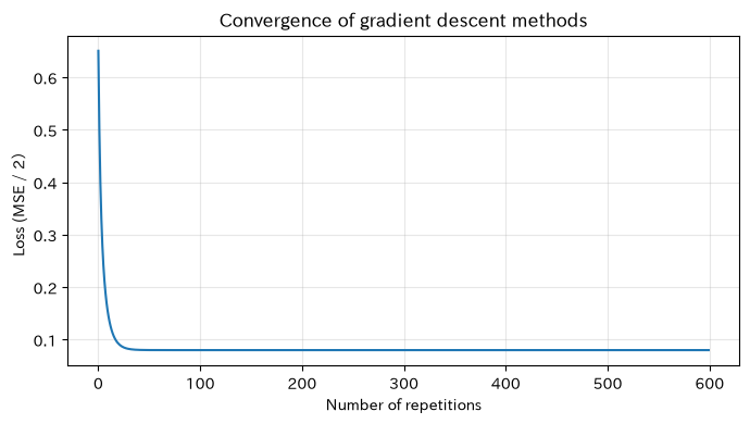
Final loss: 0.08004
Evaluation data RMSE: 0.414 μm
Reading the results
Losses decrease with iterations and converge to a certain level. When deploying on-site, not only final accuracy but also logs are made to ensure the loss curve does not oscillate or diverge, and whether improvements stopped before reaching the upper limit of iterations. If the convergence behavior changes after adding a line, it raises suspicions of changes in units, outliers, or data distribution.
No.052: Least Squares Method
Meaning in Practice
The least squares method finds a coefficient that minimizes the sum of squares between the measured and predicted values. This is a basic method for explaining and forecasting continuous KPIs such as dimensions, cycle time, and power consumption based on machining conditions.
Approach to Analysis and Modeling
The purpose is
That’s right. np.linalg.lstsq is solved using SVD, making it a numerically easier method than explicitly creating inverse matrices. RMSE can be read as the same unit as dimensional error, but it is also important to understand that it is a metric that strongly punishes large errors.
Check with Python
beta_ls, residuals, rank, singular_values = np.linalg.lstsq(X_train, y_train, rcond=None)
pred_ls = X_test @ beta_ls
rmse_ls = np.sqrt(np.mean((y_test - pred_ls) ** 2))

coef_table = pd.DataFrame({
    "item": ["slice"] + feature_cols,
    "Normalization coefficient": beta_ls,
})
display(coef_table.round(4))
print(f"Matrix rank: {rank} / {X_train.shape[1]}")
print(f"Evaluation DataRMSE: {rmse_ls:.3f} μm")| item | Normalization coefficient | |
|---|---|---|
| 0 | slice | 0.7377 |
| 1 | processing speed_rpm | 0.1792 |
| 2 | Delivery volume_mm_rev | 0.1658 |
| 3 | processing temperature_C | 0.2595 |
| 4 | vibration_mm_s | 0.1257 |
| 5 | hydraulic pressure_MPa | -0.0331 |
| 6 | tool wear | 0.3758 |
Queue rank: 7 / 7
Evaluation data RMSE: 0.414 μm
Reading the results
The absolute value of the coefficient serves as a guideline for comparing how much each standardized condition correlates with dimensional errors. However, these are correlations based on observational data and do not guarantee causal effects when processing conditions are changed. Evaluation RMSE is used to compare the resolution and tolerance range of the measuring instrument to determine whether the error is sufficient for omission of inspection or adjustment of conditions, rather than “high accuracy.”
No.053: Normal Equation
Meaning in Practice
A normal equation shows that the least squares method can be solved as a system of matrices. It is important to understand the basis for calculating coefficients and to grasp why solutions become unstable due to variables being duplicated.
Approach to Analysis and Modeling
If we set the loss gradient to 0,
You will get it. If is regular, you can write , but in implementation, the inverse matrix is not explicitly displayed and solve is used. Normal equations worsen the number of conditions, so SVD and QR decomposition are prioritized for large-scale, poor-condition problems.
Check with Python
gram = X_train.T @ X_train
rhs = X_train.T @ y_train
beta_normal = np.linalg.solve(gram, rhs)

comparison = pd.DataFrame({
    "item": ["slice"] + feature_cols,
    "lstsq": beta_ls,
    "normal equation": beta_normal,
    "poor": beta_normal - beta_ls,
})
display(comparison.round(8))
print(f"X Conditional number: {np.linalg.cond(X_train):.1f}")
print(f"X^T X Conditional number: {np.linalg.cond(gram):.1f}")| item | lstsq | normal equation | poor | |
|---|---|---|---|---|
| 0 | slice | 0.7377 | 0.7377 | 0.0 |
| 1 | processing speed_rpm | 0.1792 | 0.1792 | 0.0 |
| 2 | Delivery volume_mm_rev | 0.1658 | 0.1658 | 0.0 |
| 3 | processing temperature_C | 0.2595 | 0.2595 | -0.0 |
| 4 | vibration_mm_s | 0.1257 | 0.1257 | -0.0 |
| 5 | hydraulic pressure_MPa | -0.0331 | -0.0331 | 0.0 |
| 6 | tool wear | 0.3758 | 0.3758 | 0.0 |
Number of X conditions: 4.4
Number of X^T X conditions: 19.1
Reading the results
In this data, the coefficients for both methods are almost identical. On the other hand, the number of conditions for is greater than . In practice, formulas are only theoretically correct and not adopted; instead, the number of variables, correlations, and accuracy requirements are checked. If the number of conditions surges after adding an explanatory variable, review whether the KPI contains new information.
No.054: Ridge Returns
Meaning in Practice
If you include similar variables such as equipment settings and actual measurements, or the original sensor and derived KPIs at the same time, the regression coefficient can fluctuate significantly. Ridge regression reduces coefficients and stabilizes forecasting and operations.
Approach to Analysis and Modeling
Ridge’s return
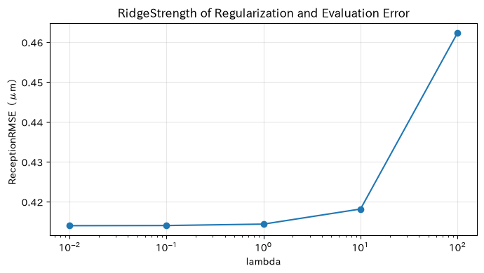
Solve the problem and it becomes . Here, we add almost the same derivative metrics to the feed volume, intentionally strengthening the correlation. Intercepts are not regularized. is selected based on evaluation data or cross-validation.
Check with Python
feed_proxy = X_std[:, 1] + np.random.default_rng(0).normal(0, 0.001, n)
X_col = np.column_stack([X, feed_proxy])
Xc_train, Xc_test = X_col[train_idx], X_col[test_idx]
penalty = np.eye(Xc_train.shape[1])
penalty[0, 0] = 0

ridge_rows = []
ridge_models = {}
for lam in [0, 0.01, 0.1, 1, 10, 100]:
    beta = np.linalg.solve(Xc_train.T @ Xc_train + lam * penalty, Xc_train.T @ y_train)
    ridge_models[lam] = beta
    ridge_rows.append({
        "lambda": lam,
        "ReceptionRMSE": np.sqrt(np.mean((y_test - Xc_test @ beta) ** 2)),
        "coefficient norm": np.linalg.norm(beta[1:]),
        "feed rate coefficient": beta[2],
        "Derived feeding coefficient": beta[-1],
    })

ridge_result = pd.DataFrame(ridge_rows)
display(ridge_result.round(4))

plt.figure(figsize=(7, 4))
plt.semilogx(ridge_result.loc[1:, "lambda"], ridge_result.loc[1:, "ReceptionRMSE"], marker="o")
plt.title("RidgeStrength of Regularization and Evaluation Error")
plt.xlabel("lambda")
plt.ylabel("ReceptionRMSE(μm)")
plt.grid(True, alpha=0.3)
plt.tight_layout()
plt.show()| lambda | ReceptionRMSE | coefficient norm | feed rate coefficient | Derived feeding coefficient | |
|---|---|---|---|---|---|
| 0 | 0.00 | 0.4139 | 10.4952 | -7.3286 | 7.4956 |
| 1 | 0.01 | 0.4140 | 0.5279 | 0.0223 | 0.1436 |
| 2 | 0.10 | 0.4140 | 0.5207 | 0.0769 | 0.0891 |
| 3 | 1.00 | 0.4144 | 0.5186 | 0.0833 | 0.0845 |
| 4 | 10.00 | 0.4182 | 0.5000 | 0.0906 | 0.0907 |
| 5 | 100.00 | 0.4624 | 0.3881 | 0.1064 | 0.1064 |
Reading the results
Without regularization, coefficients are unstably distributed to almost the same two feed indicators. A moderate ridge maintains evaluation error while suppressing the coefficient norm. that is too large will shrink to the required signal. When explaining coefficients as causal contributions, even with Ridge, you can organize the meaning of duplicate variables and record the selected and evaluation methods.
No.055: Logistic Regression
Meaning in Practice
Not only can it directly predict the binary values of defective and good products, but by outputting it as defect probability, multiple operational thresholds such as full inspection, additional inspection, and normal shipment can be designed.
Approach to Analysis and Modeling
Logistic regression is
represents the defect probability. We minimize cross-entropy loss and learn here using gradient descent. The probability threshold is not fixed at 0.5, but is determined by missed costs, additional inspection capacity, and defect rates.
Check with Python
def sigmoid(z):
    z = np.clip(z, -30, 30)
    return 1 / (1 + np.exp(-z))

beta_logit = np.zeros(X_train.shape[1])
logloss_history = []
for _ in range(1500):
    p = sigmoid(X_train @ beta_logit)
    logloss = -np.mean(y_cls[train_idx] * np.log(p + 1e-12) + (1 - y_cls[train_idx]) * np.log(1 - p + 1e-12))
    logloss_history.append(logloss)
    beta_logit -= 0.08 * (X_train.T @ (p - y_cls[train_idx]) / len(train_idx))

p_test = sigmoid(X_test @ beta_logit)
threshold = 0.35
pred_cls = (p_test >= threshold).astype(int)
cm = confusion_matrix(y_cls[test_idx], pred_cls)
tn, fp, fn, tp = cm.ravel()

metrics = pd.Series({
    "AUC": roc_auc_score(y_cls[test_idx], p_test),
    "Recall (Poor Capture Rate)": tp / (tp + fn),
    "Compatibility rate": tp / (tp + fp),
    "Additional testing rate": pred_cls.mean(),
})
display(metrics.to_frame("value").round(3))
display(pd.DataFrame(cm, index=["In fact,_good product", "In fact,_bad"], columns=["Prediction_good product", "Prediction_bad"]))| value | |
|---|---|
| AUC | 0.776 |
| Recall (Poor Capture Rate) | 0.533 |
| Compatibility rate | 0.615 |
| Additional testing rate | 0.217 |
| Prediction_good product | Prediction_bad | |
|---|---|---|
| In fact,_good product | 40 | 5 |
| In fact,_bad | 7 | 8 |
Reading the results
AUC represents the lot’s risk ranking ability, recall rate indicates how many actual defects were picked up, and accuracy rate represents the efficiency of additional inspections. The threshold of 0.35 is designed to cover a wider range of inspection targets and minimize missed opportunities. In practice, indicators fluctuate during periods with fewer defects, so confidence intervals, product type evaluation, probability calibration, and inspection load after threshold changes are checked together.
No.056: Newton Method
Meaning in Practice
The Newton method adjusts the update width not only by gradient but also by using the curvature of the loss function. While reducing the number of iterations, each update solves simultaneous equations, so when there are many variables, it is necessary to design computational load and stability.
Approach to Analysis and Modeling
Using gradient and Hessian matrix ,
I will update you. In logistic regression, and are used. In the implementation, instead of creating an inverse matrix, solve is used, and small diagonal terms are added for numerical stability.
Check with Python
beta_newton = np.zeros(X_train.shape[1])
newton_history = []

for iteration in range(10):
    p = sigmoid(X_train @ beta_newton)
    loss = -np.mean(y_cls[train_idx] * np.log(p + 1e-12) + (1 - y_cls[train_idx]) * np.log(1 - p + 1e-12))
    newton_history.append(loss)
    gradient = X_train.T @ (p - y_cls[train_idx])
    weights = p * (1 - p)
    hessian = X_train.T @ (weights[:, None] * X_train) + 1e-6 * np.eye(X_train.shape[1])
    beta_newton -= np.linalg.solve(hessian, gradient)

display(pd.DataFrame({
    "Repeatedly": np.arange(1, len(newton_history) + 1),
    "Newtonloss of law": newton_history,
}).round(6))
print(f"Final Loss of the Slope Descent Method: {logloss_history[-1]:.6f}")
print(f"NewtonFinal loss of law: {newton_history[-1]:.6f}")| Repeatedly | Newtonloss of law | |
|---|---|---|
| 0 | 1 | 0.6931 |
| 1 | 2 | 0.3831 |
| 2 | 3 | 0.3437 |
| 3 | 4 | 0.3378 |
| 4 | 5 | 0.3376 |
| 5 | 6 | 0.3376 |
| 6 | 7 | 0.3376 |
| 7 | 8 | 0.3376 |
| 8 | 9 | 0.3376 |
| 9 | 10 | 0.3376 |
Final loss by gradient descent: 0.337600
Newton Act final loss: 0.337592
Reading the results
The Newton method reduces losses with fewer iterations. However, having “fewer iterations” does not mean “shorter computation times.” In models with many variables, creating and solving Hessian matrices becomes dominant. If data is nearly completely separated or explanatory variables overlap, it becomes unstable, so regularization and stepwidth control are combined.
No.057: Hessian Matrix
Meaning in Practice
The Hessian matrix represents how much the loss bends in each direction of each parameter. Small eigenvalue directions are where it is difficult to identify coefficients from the data, and estimates can easily fluctuate with slight data changes.
Approach to Analysis and Modeling
A Hessian matrix is a matrix arranged with second-order partial derivatives
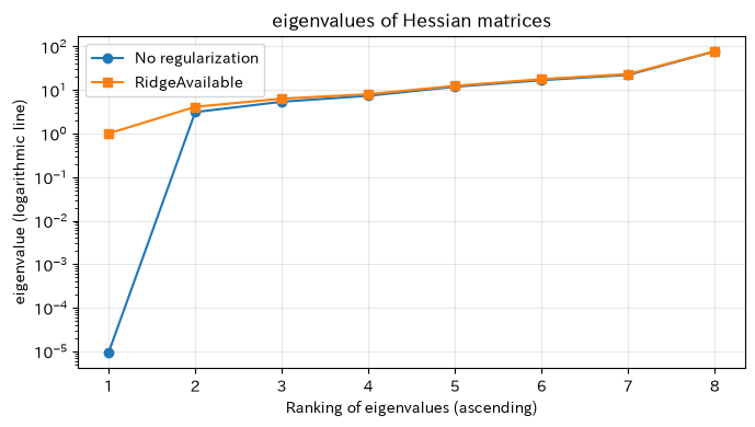
That’s right. If all eigenvalues are positive, it is locally convex. If the ratio of maximum eigenvalues to minimum eigenvalues is large, the curvature difference in each direction becomes larger, making optimization more difficult. The diagonal term of Ridge pushes up small eigenvalues.
Check with Python
p_col = sigmoid(Xc_train @ np.pad(beta_newton, (0, 1)))
W_col = p_col * (1 - p_col)
H_col = Xc_train.T @ (W_col[:, None] * Xc_train)
H_ridge = H_col + 1.0 * penalty

eig_plain = np.linalg.eigvalsh(H_col)
eig_ridge = np.linalg.eigvalsh(H_ridge)
hessian_table = pd.DataFrame({
    "indicator": ["Minimum eigenvalue", "maximum eigenvalue", "Conditional number"],
    "No regularization": [eig_plain.min(), eig_plain.max(), np.linalg.cond(H_col)],
    "RidgeAvailable": [eig_ridge.min(), eig_ridge.max(), np.linalg.cond(H_ridge)],
})
display(hessian_table.round(4))

plt.figure(figsize=(7, 4))
plt.semilogy(np.arange(1, len(eig_plain) + 1), eig_plain, marker="o", label="No regularization")
plt.semilogy(np.arange(1, len(eig_ridge) + 1), eig_ridge, marker="s", label="RidgeAvailable")
plt.title("eigenvalues of Hessian matrices")
plt.xlabel("Ranking of eigenvalues (ascending)")
plt.ylabel("eigenvalue (logarithmic line)")
plt.grid(True, alpha=0.3)
plt.legend()
plt.tight_layout()
plt.show()| indicator | No regularization | RidgeAvailable | |
|---|---|---|---|
| 0 | Minimum eigenvalue | 0.0000e+00 | 1.0000 |
| 1 | maximum eigenvalue | 7.6713e+01 | 77.5857 |
| 2 | Conditional number | 8.1267e+06 | 77.5850 |
Reading the results
Including a nearly overlapping stroke indicator reduces the minimum eigenvalue and creates a flat direction on the loss plane. Ridge adds curvature in that direction to improve the number of conditions. In practice, deterioration in the number of conditions is not treated merely as a calculation problem, but as a data design issue involving “whether KPIs with almost the same meaning are being managed redundantly” or “whether independent test conditions are lacking.”
No.058: Conjugate Gradient Method
Meaning in Practice
As the number of devices, varieties, and features increases, the cost of directly decomposing the matrix of simultaneous equations rises. The conjugate gradient method finds the solution for symmetric positive definite matrices by iterating the matrix vector product without creating an inverse matrix.
Approach to Analysis and Modeling
Normal Equations of Ridge Regression
becomes a symmetric positive definite value through regularization. The conjugate gradient method uses conjugate search directions to efficiently minimize quadratic forms. Residual is used for convergence determination.
Check with Python
def conjugate_gradient(A, b, tol=1e-10, max_iter=100):
    x = np.zeros_like(b)
    r = b - A @ x
    p = r.copy()
    residual_norms = [np.linalg.norm(r)]
    for _ in range(max_iter):
        Ap = A @ p
        alpha = (r @ r) / (p @ Ap)
        x = x + alpha * p
        r_new = r - alpha * Ap
        residual_norms.append(np.linalg.norm(r_new))
        if residual_norms[-1] < tol:
            break
        beta = (r_new @ r_new) / (r @ r)
        p = r_new + beta * p
        r = r_new
    return x, residual_norms

lam = 1.0
A_cg = Xc_train.T @ Xc_train + lam * penalty
b_cg = Xc_train.T @ y_train
beta_cg, cg_residuals = conjugate_gradient(A_cg, b_cg)
beta_direct = np.linalg.solve(A_cg, b_cg)

print(f"Number of repetitions: {len(cg_residuals) - 1}")
print(f"Difference from the direct method: {np.linalg.norm(beta_cg - beta_direct):.3e}")

plt.figure(figsize=(7, 4))
plt.semilogy(cg_residuals, marker="o")
plt.title("Residual Convergence of Conjugate Gradient Method")
plt.xlabel("Number of repetitions")
plt.ylabel("residual norm")
plt.grid(True, alpha=0.3)
plt.tight_layout()
plt.show()
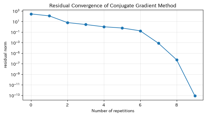
Number of repetitions: 9
Difference from direct method: 1.491e-14
Reading the results
The residual decreases with fewer iterations, yielding a solution close to the direct method. For this small matrix, the direct method is sufficient, but the conjugate gradient method is effective for large-scale problems where it is difficult to explicitly hold the matrix. In practice, we manage positive statability, tolerance of error, maximum iteration, and whether preprocessing is used, and design operations that do not deliver old coefficients before convergence.
No.059: Kernel Method
Meaning in Practice
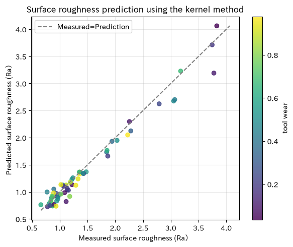
Surface roughness can suddenly deteriorate in areas where temperature or vibration deviate from the standard, or where both are high. The kernel method does not explicitly create numerous nonlinear features from the original variable, but instead makes nonlinear predictions based on relationships between similar operating conditions.
Approach to Analysis and Modeling
RBF Kernel
Create a similarity matrix between learning points. At Kernel Ridge,
and predict from the kernel value with the new point. controls the scope of influence, controls smoothness, and extrapolation outside the learning area is handled with care.
Check with Python
kernel_cols = [2, 3]  # Processing temperature and vibration after standardization
Z_train = X_std[train_idx][:, kernel_cols]
Z_test = X_std[test_idx][:, kernel_cols]

def rbf_kernel(A, B, gamma=0.7):
    sq_dist = ((A[:, None, :] - B[None, :, :]) ** 2).sum(axis=2)
    return np.exp(-gamma * sq_dist)

rough_train = df.loc[train_idx, "surface roughness_Ra"].to_numpy()
rough_test = df.loc[test_idx, "surface roughness_Ra"].to_numpy()
K_train = rbf_kernel(Z_train, Z_train, gamma=0.1)
alpha = np.linalg.solve(K_train + 0.01 * np.eye(len(train_idx)), rough_train)
pred_kernel = rbf_kernel(Z_test, Z_train, gamma=0.1) @ alpha

Z_linear = np.column_stack([np.ones(len(train_idx)), Z_train])
coef_linear = np.linalg.lstsq(Z_linear, rough_train, rcond=None)[0]
pred_linear_2d = np.column_stack([np.ones(len(test_idx)), Z_test]) @ coef_linear

kernel_compare = pd.DataFrame({
    "Model": ["Linear Regression of Temperature and Vibration", "RBF Kernel Ridge"],
    "ReceptionRMSE": [
        np.sqrt(np.mean((rough_test - pred_linear_2d) ** 2)),
        np.sqrt(np.mean((rough_test - pred_kernel) ** 2)),
    ],
})
display(kernel_compare.round(4))

plt.figure(figsize=(6, 5))
plt.scatter(rough_test, pred_kernel, c=df.loc[test_idx, "tool wear"], cmap="viridis", alpha=0.8)
limits = [min(rough_test.min(), pred_kernel.min()), max(rough_test.max(), pred_kernel.max())]
plt.plot(limits, limits, "--", color="gray", label="Measured=Prediction")
plt.title("Surface roughness prediction using the kernel method")
plt.xlabel("Measured surface roughness (Ra)")
plt.ylabel("Predicted surface roughness (Ra)")
plt.grid(True, alpha=0.3)
plt.colorbar(label="tool wear")
plt.legend()
plt.tight_layout()
plt.show()| Model | ReceptionRMSE | |
|---|---|---|
| 0 | Linear Regression of Temperature and Vibration | 0.8336 |
| 1 | RBF Kernel Ridge | 0.1498 |
Reading the results
The kernel method captures the curved relationship between temperature and vibration, reducing surface roughness evaluation error compared to linear regression with the same two variables. However, these two variables alone can still affect factors like tool wear. If you notice uneven wear in color, this is an additional candidate. It is necessary to detect conditions outside the training data without increasing variables solely by improving accuracy, and to hold forecasts outside the applicable scope.
No.060:Attention
Meaning in Practice
If there is a large amount of time series data during a single batch of processing, simply averaging all points with the same weight can dilute the short time with strong abnormal signs. Attention assigns significant weight to points relevant to the current decision-making purpose.
Approach to Analysis and Modeling
Scaled Dot-Product Attention
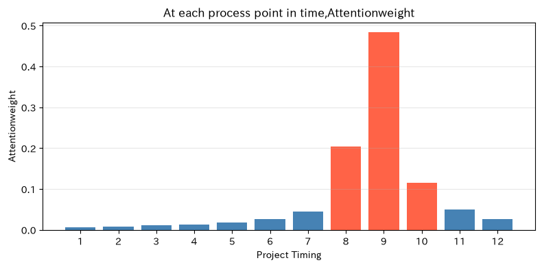
That’s right. indicates the state you want to find, shows the characteristics at each point in time, and represents the information you want to consolidate. Here, instead of using a trained Transformer, we use a simplified example querying high temperature, vibration, and load to confirm the meaning of weight. Weight does not prove a causal cause of failure.
Check with Python
stages = np.arange(1, 13)
stage_temp = np.array([59.8, 60.2, 60.7, 61.0, 61.4, 62.0, 62.6, 63.7, 64.2, 63.4, 62.8, 62.1])
stage_vib = np.array([1.20, 1.24, 1.28, 1.31, 1.35, 1.42, 1.51, 1.82, 2.05, 1.72, 1.55, 1.44])
stage_load = np.array([0.40, 0.43, 0.48, 0.52, 0.56, 0.61, 0.67, 0.91, 1.00, 0.78, 0.65, 0.55])

stage_matrix = np.column_stack([stage_temp, stage_vib, stage_load])
keys = (stage_matrix - stage_matrix.mean(axis=0)) / stage_matrix.std(axis=0)
query = np.array([0.7, 1.0, 0.6])
scores = keys @ query / np.sqrt(keys.shape[1])
weights = np.exp(scores - scores.max())
weights /= weights.sum()
values = 0.4 * keys[:, 0] + 0.8 * keys[:, 1] + 0.5 * keys[:, 2]
attention_summary = weights @ values

attention_table = pd.DataFrame({
    "Project Timing": stages, "temperature_C": stage_temp, "vibration_mm_s": stage_vib,
    "load index": stage_load, "Attentionweight": weights,
}).sort_values("Attentionweight", ascending=False)
display(attention_table.head(5).round(4))
print(f"AttentionRisk expressions summarized in: {attention_summary:.3f}")

plt.figure(figsize=(8, 4))
plt.bar(stages, weights, color=np.where(weights >= np.quantile(weights, 0.75), "tomato", "steelblue"))
plt.title("At each process point in time,Attentionweight")
plt.xlabel("Project Timing")
plt.ylabel("Attentionweight")
plt.xticks(stages)
plt.grid(True, axis="y", alpha=0.3)
plt.tight_layout()
plt.show()| Project Timing | temperature_C | vibration_mm_s | load index | Attentionweight | |
|---|---|---|---|---|---|
| 8 | 9 | 64.2 | 2.05 | 1.00 | 0.4829 |
| 7 | 8 | 63.7 | 1.82 | 0.91 | 0.2036 |
| 9 | 10 | 63.4 | 1.72 | 0.78 | 0.1143 |
| 10 | 11 | 62.8 | 1.55 | 0.65 | 0.0498 |
| 6 | 7 | 62.6 | 1.51 | 0.67 | 0.0444 |
Risk expression summarized by Attention: 2.309
Reading the results
At process points where temperature, vibration, and load rise simultaneously, significant weight is added, allowing staff to narrow down candidates for waveform inspection. However, this weight depends on the query you set. The practical Attention model examines biases, masking, sensor defects, process lengths by product type, and differences in weight and prediction contributions, then reviews them alongside the original waveform.
Practical Implications Seen Through Target Exercise
- Classifying methods by objective variables: For dimensional errors, select the least square; for defect probability, select the loss function from the on-site decision-making format, such as the least square; for defect probability, Logistic regression.
- Quality control for convergence and stability: Record gradients, losses, residuals, number of conditions, and eigenvalues of the Hessian matrix; simply obtaining a value does not count as a normal termination.
- strongly correlatedKPIOrganize: Ridge is effective for stabilization, but it is not a reason to leave duplicate metric business definitions unaddressed.
- Scope management is necessary for non-linearization.: While kernel methods capture complex quality relationships, they pay attention to extrapolation and explainability beyond the learning scope.
- Attentionis a guide line that narrows down the points of confirmation.: Instead of using weight to determine the cause, it connects to the original sensor, maintenance history, and actual item verification.
What is necessary for practical implementation
1. Define the purpose of the judgment and the loss
Dimensional forecasting, additional inspections, condition recommendations, and equipment shutdowns all contribute to the cost of errors. Missed cases, over-detections, inspection man-hours, and downtime losses are organized, and success is determined not only by RMSE and AUC but also by operational KPIs.
2. Managing Data Lineage and Segmentation
It links equipment, varieties, tools, material lots, workers, maintenance history, and instrument calibration. To avoid mixing in future information, we conduct verification across chronological sequences, equipment, and product types.
3. Monitor numerical calculations
Standardization criteria, missing processing, regularization factors, convergence conditions, and library versions are fixed. Include the number of conditions, number of iterations, residuals, and flags outside the prediction range as monitoring items in the model.
4. Connect to the site flow
Determine the number of test targets, responsible departments, confirmation deadlines, and lifting conditions for each probability threshold. Attention Weights and coefficients are displayed along with the source data, allowing personnel to track the basis.
5. Define the division of responsibility after the PoC
Clarify who is responsible for data quality, model updates, threshold approvals, equipment shutdown decisions, and audit logs. We also prepare for degenerate driving when model performance declines and for reverting to old rules.
Conclusion
From No.051 to No.060, starting with gradient descent and least squares methods, we examined normal equations, Ridge regression, logistic regression, Newton’s method, Hessian matrix, conjugate gradient method, kernel method, and attention as one of the manufacturing quality decision stories.
Matrix calculation is not just a technique for creating predicted values. By visualizing convergence, curvature, correlation, regularization, similarity, and weighting at point in time, it becomes a tool for sharing What results to trust under what conditions, and what to check next? within the organization.
Consultations for Corporations
At Suri Kobo, we support quality forecasting, defect factor analysis, machining condition optimization, equipment data utilization, model numerical stability evaluation, and the transition from PoC to on-site operations in manufacturing. Even at a stage where the location and purpose of data are not yet organized, you can consult with us starting from inventory of business challenges.
📩 Contact Us: surikobo.co.jp/contact
Please feel free to consult us first.