Connecting processing data to decision-making quickly, accurately, and reproducibly

CuPy, JAX, Polars, Speed, Notebook Practice: 100 Exercises No.091–No.100

When utilizing data on the manufacturing floor, simply speeding up calculations is not enough. Even if equipment, days, and shifts increase, processing can continue, the same results can be reproduced from the same input, and only when numerical errors and processing times can be explained can it be incorporated into daily inspection decisions. In this article, we will use a fictional machining line as the subject and treat From selecting computing platforms to speed, visualization, verification, and prioritizing inspections as a single flow.

[!NOTE] This material is a notebook previously used by Surikoubo (or personally by the representative, Kazuyama), and has been reconstructed, edited, and published with the company’s permission.
All data listed is fictional and has no relation whatsoever to real companies, factories, or figures.

Introduction: Practical Challenges in Manufacturing Covered in This Article

In a hypothetical factory, temperature, vibration, power consumption, processing time, and quality score are recorded for each processing cycle. While we want to aggregate the previous day’s data and recommend inspection recommendations before the morning meeting, the expansion of facilities has extended processing times, the notebook results differ for each person in charge, and there is a lack of validation after changing the calculation method.

Therefore, we estimate processing volume and computational resources, accelerate table processing and matrix calculations where appropriate, and retain reproducible analysis records and verification metrics. The ultimate goal is not to adopt libraries, but to Allocate limited inspection man-hours to equipment with high risks of shutdown or defects.

Common situations on site

• The tally that took only a few seconds during prototyping became too late for the morning meeting as it was deployed at all factories.
• GPU and parallelization were introduced, but when considering transfer and boot costs, it didn’t get faster.
• Creating report values without running the notebook from above, leaving old variables intact.
• Cannot detect rounding errors or missing processing before or after speeding up
• Measuring only average processing time and overlooking daily variation and worst-case times
• While there are many graphs, inspection targets and criteria are not clearly stated.

Why is this issue so difficult to judge?

Processing time depends not only on the number of data entries but also on matrix shape, data type, memory access, transfer, compilation, and parallel granularity. Even on a foundation with theoretically high computational performance, the preparation cost dominates for small processing. Also, if the order of operations changes due to speed, the floating-point results will not be exactly the same.

Therefore, speed is not evaluated by a single value, but the total travel time

$$T_{\mathrm{total}}=T_{\mathrm{read}}+T_{\mathrm{prepare}}+T_{\mathrm{transfer}}+T_{\mathrm{compute}}+T_{\mathrm{report}}$$

It is also necessary to simultaneously evaluate tolerance of error, reproducibility, and maintainability.

Overview of Exercise covered this time

No.	Theme	Judgment in the manufacturing industry
091	CuPy	Estimating adoption effects including GPU transfer
092	JAX	Using pure functions, batch calculations, and differentiation for model verification
093	Polars	Aggregate large amounts of machining performance using delayed and column-oriented methods
094	Accelerated matrix computation	Vectorize loops and reduce unnecessary intermediate arrays
095	parallelization	Determining the Granularity of Equipment-Specific Processing That Can Be Divided
096	Utilizing Notebooks	Leave parameters, validation, and execution trails
097	visualization	Translating anomalies into inspection priority
098	numerical error	Detecting Errors and Adverse Conditions to Prevent Misjudgment
099	Benchmark	Fairly iterate the candidate implementations
100	The World of Matrix Computing	Integrating technology choices to create operational plans

Preparing the Python environment

NumPy performs matrix calculations, pandas and Polars handle table processing, and Matplotlib provides visualization. CuPy and JAX are heavily dependent on GPU and accelerator environments, so they are not mandatory; they are detected whenever available. The random number generator is fixed at np.random.default_rng(91).

%matplotlib inline
%config InlineBackend.figure_format = 'svg'

import hashlib
import importlib.util
import platform
import sys
import time
from concurrent.futures import ThreadPoolExecutor

import japanize_matplotlib
import matplotlib
import matplotlib.pyplot as plt
import numpy as np
import pandas as pd
import polars as pl
from IPython.display import display

rng = np.random.default_rng(91)
plt.rcParams["figure.figsize"] = (8, 4.5)

print(f"Python     : {sys.version.split()[0]}")
print(f"NumPy      : {np.__version__}")
print(f"pandas     : {pd.__version__}")
print(f"Polars     : {pl.__version__}")
print(f"Matplotlib : {matplotlib.__version__}")
print(f"OS          : {platform.system()} {platform.machine()}")
print("CuPy       :", "Available" if importlib.util.find_spec("cupy") else "Not yet implemented (CPUReproduced in this way)")
print("JAX        :", "Available" if importlib.util.find_spec("jax") else "Not yet implemented (NumPyReproducing the principle in this way)")

Python     : 3.13.1
NumPy      : 2.5.1
pandas     : 3.0.3
Polars     : 1.42.1
Matplotlib : 3.11.0
OS          : Darwin arm64
CuPy: Not installed (reproduced on CPU)
JAX: Not installed (principle reproduced with NumPy)

Creation of Fictional Data

For 4 lines and 12 facilities, we generate virtual data for 20 cycles of each facility over 60 days. Aging trends, night shift loads, and equipment-specific differences are reflected in temperature, vibration, power consumption, and cycle time, and from these, defect flags are created. From then on, the same data was used for all subsequent exercises to align the premise for technical comparison.

In practice, equipment ID, time, unit, calibration history, and reason for missing are managed as data contracts, distinguishing between “unmeasured” and normal values of zero.

lines = [f"Line{i}" for i in range(1, 5)]
equipment = [f"Equipment{i:02d}" for i in range(1, 13)]
n_days, cycles_per_equipment = 60, 20
n = n_days * len(equipment) * cycles_per_equipment

day = np.repeat(np.arange(n_days), len(equipment) * cycles_per_equipment)
equipment_id = np.tile(np.repeat(np.arange(len(equipment)), cycles_per_equipment), n_days)
shift = np.tile(np.arange(cycles_per_equipment) % 2, n_days * len(equipment))
line_id = equipment_id // 3
age = np.array([2, 5, 8, 3, 7, 11, 4, 9, 6, 12, 3, 10])[equipment_id]
load = np.clip(rng.normal(0.72 + 0.05 * shift, 0.09, n), 0.35, 1.0)
temperature = 43 + 13 * load + 0.18 * age + 0.025 * day + rng.normal(0, 1.7, n)
vibration = 1.3 + 1.4 * load + 0.09 * age + 0.012 * day + rng.normal(0, 0.28, n)
power = 14 + 22 * load + 0.35 * line_id + rng.normal(0, 1.4, n)
cycle_sec = 48 + 13 * load + 0.25 * age + rng.normal(0, 2.2, n)
quality_score = 100 - 0.30 * (temperature - 50) - 2.4 * (vibration - 2.5) - rng.normal(0, 1.0, n)
logit = -5.2 + 0.075 * (temperature - 50) + 0.85 * (vibration - 2.5) + 0.55 * shift
defect_prob = 1 / (1 + np.exp(-logit))
defect = rng.binomial(1, defect_prob)

production_df = pd.DataFrame({
    "days": day + 1, "Line": np.array(lines)[line_id], "Equipment": np.array(equipment)[equipment_id],
    "Shift": np.where(shift == 0, "daytime", "night"), "load factor": load, "temperature_C": temperature,
    "vibration_mm_s": vibration, "power consumption_kW": power, "cycle second": cycle_sec,
    "Quality score": quality_score, "bad": defect,
})
features = ["load factor", "temperature_C", "vibration_mm_s", "power consumption_kW", "cycle second"]
X = production_df[features].to_numpy(dtype=np.float64)
Xz = (X - X.mean(axis=0)) / X.std(axis=0)

display(production_df.head().style.format({c: "{:.2f}" for c in features + ["Quality score"]}))
print(f"Number of records: {len(production_df):,} / matrix shape: {Xz.shape} / defect rate: {defect.mean():.2%}")

	days	Line	Equipment	Shift	load factor	temperature_C	vibration_mm_s	power consumption_kW	cycle second	Quality score	bad
0	1	Line1	Equipment01	daytime	0.73	54.11	2.50	31.38	63.65	99.56	0
1	1	Line1	Equipment01	night	0.84	54.58	2.99	32.46	58.95	96.96	0
2	1	Line1	Equipment01	daytime	0.60	51.38	2.02	27.15	58.40	100.27	0
3	1	Line1	Equipment01	night	0.72	52.40	1.92	31.06	54.44	99.91	0
4	1	Line1	Equipment01	daytime	0.77	52.37	2.72	30.02	59.08	97.88	0

Number of records: 14,400 / Matrix shape: (14400, 5) / Defect rate: 2.28%

---

No.091：CuPy

Meaning in Practice

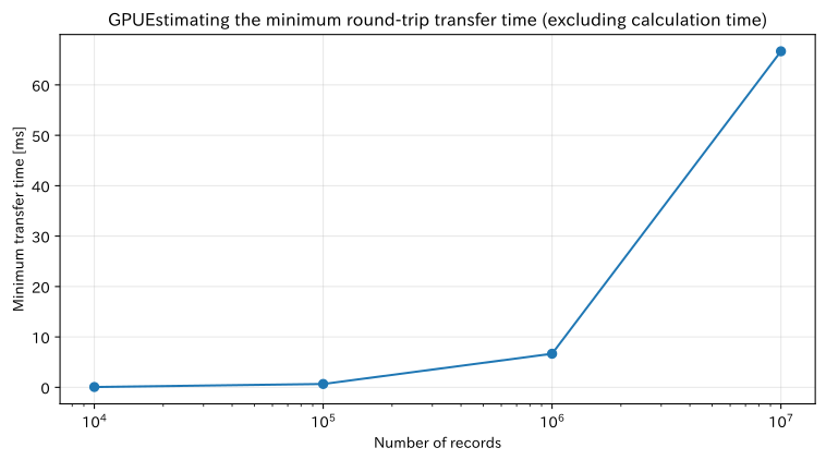
CuPy performs array computation on NVIDIA GPUs using notation similar to NumPy. It is a candidate when repeating large numbers of waveform features, images, and simulations using the same matrix operations. However, if you send it to the GPU and return it immediately, the transfer time will negate the benefits.

Approach to Analysis and Modeling

If the data volume crossing the CPU and GPU boundary is $B$ and the transfer bandwidth is $W$, the lower bound of round-trip transfer time is approximately $2B/W$. Here, the same risk score is calculated by switching the array API called xp, and in environments without a physical GPU, it safely falls back to NumPy. At the time of recruitment, the end-to-end time after warm-up is measured.

Check with Python

try:
    import cupy as cp
    xp, backend = cp, "CuPy (GPU)"
except ImportError:
    xp, backend = np, "NumPy (CPU fallback)"

weights = xp.asarray([0.25, 0.20, 0.30, 0.10, 0.15])
X_device = xp.asarray(Xz)
risk_device = X_device @ weights
risk_091 = cp.asnumpy(risk_device) if backend.startswith("CuPy") else np.asarray(risk_device)

sizes = np.array([10_000, 100_000, 1_000_000, 10_000_000])
bytes_roundtrip = sizes * len(features) * 8 * 2
transfer_plan = pd.DataFrame({
    "Number of lines": sizes, "Round-trip data volume_MB": bytes_roundtrip / 1e6,
    "Lower transfer limit_ms_band12GBevery second": bytes_roundtrip / 12e9 * 1e3,
})
print("Execution Backend:", backend)
display(transfer_plan.style.format({"Round-trip data volume_MB": "{:.1f}", "Lower transfer limit_ms_band12GBevery second": "{:.2f}"}))

plt.plot(sizes, transfer_plan["Lower transfer limit_ms_band12GBevery second"], marker="o")
plt.xscale("log")
plt.title("GPUEstimating the minimum round-trip transfer time (excluding calculation time)")
plt.xlabel("Number of records")
plt.ylabel("Minimum transfer time [ms]")
plt.grid(True, alpha=0.3)
plt.tight_layout()
plt.show()

Execution Backend: NumPy (CPU fallback)

	Number of lines	Round-trip data volume_MB	Lower transfer limit_ms_band12GBevery second
0	10000	0.8	0.07
1	100000	8.0	0.67
2	1000000	80.0	6.67
3	10000000	800.0	66.67

Reading the results

The execution backend for this time is explicitly displayed, allowing the same computational results to be reproduced even without a GPU. The estimate is not a value that proves GPU dominance, but the minimum time needed for transfer alone. In practice, the array is kept on the GPU to consolidate multiple processes, and the total time including CPU preprocessing and report creation, GPU memory, and operational costs are compared.

---

No.092：JAX

Meaning in Practice

JAX can JIT compile functions similar to NumPy and convert them into automatic differentiation or batch vectorization. It is effective for repeatedly evaluating the same function in quality prediction parameter adjustments or multi-condition simulations.

Approach to Analysis and Modeling

Easy-to-convert calculations describe the external state as pure functions without rewriting them. Here, the analytical gradient $\nabla L=X^\mathsf{T}(\sigma(Xw)-y)/n$ of logistic loss $L(w)$ is compared to finite difference. When introducing JAX, this function is targeted for jit, grad, and vmap, and measurements are taken separately from the first compilation and subsequent cycles.

Check with Python

X_jax = np.column_stack([np.ones(len(Xz)), Xz])
y_jax = defect.astype(float)

def logistic_loss(w, X_input=X_jax, y_input=y_jax):
    z = X_input @ w
    return np.mean(np.logaddexp(0, z) - y_input * z)

def analytic_gradient(w):
    z = X_jax @ w
    p = 1 / (1 + np.exp(-z))
    return X_jax.T @ (p - y_jax) / len(y_jax)

w0 = np.zeros(X_jax.shape[1])
eps = 1e-6
grad_fd = np.array([(logistic_loss(w0 + eps * np.eye(len(w0))[j]) -
                     logistic_loss(w0 - eps * np.eye(len(w0))[j])) / (2 * eps)
                    for j in range(len(w0))])
grad_an = analytic_gradient(w0)
gradient_check = pd.DataFrame({"coefficient": ["slice"] + features, "analytical gradient": grad_an, "finite difference": grad_fd,
                               "absolute difference": np.abs(grad_an - grad_fd)})
display(gradient_check.style.format({"analytical gradient": "{:.6f}", "finite difference": "{:.6f}", "absolute difference": "{:.2e}"}))
print("Maximum error in gradient check:", f"{np.max(np.abs(grad_an-grad_fd)):.2e}")

	coefficient	analytical gradient	finite difference	absolute difference
0	slice	0.477153	0.477153	9.97e-11
1	load factor	-0.008225	-0.008225	4.26e-11
2	temperature_C	-0.009080	-0.009080	4.42e-12
3	vibration_mm_s	-0.010062	-0.010062	6.76e-11
4	power consumption_kW	-0.008843	-0.008843	2.26e-11
5	cycle second	-0.006579	-0.006579	1.38e-11

Maximum gradient check error: 9.97e-11

Reading the results

The analysis gradient and finite difference matched with sufficiently small errors, allowing us to inspect the implementation of the loss function to be converted. JAX further improves maintainability with automatic differentiation, managing initial JIT costs, recompilation due to array shape changes, random number keys, and 64-bit settings, while also recording not only training results but also gradient checks for testing.

---

No.093：Polars

Meaning in Practice

Polars features column-oriented, parallel execution, and delayed evaluation, making it suitable for extracting and aggregating large volumes of machining performance. Shorten the pre-processing of morning meeting KPIs, giving analysts more time to study models.

Approach to Analysis and Modeling

Select the required columns, narrow down rows, and aggregate by equipment as a single delayed query and execute it at the last collect(). In practice, Parquet’s column and row group reduction is effective, so conclusions are not drawn based solely on CSV load comparisons. First, verify that the aggregation definition matches the pandas version.

Check with Python

pl_df = pl.DataFrame(production_df.to_dict(orient="list"))
summary_pl = (
    pl_df.lazy()
    .filter(pl.col("days") > 30)
    .group_by(["Line", "Equipment"])
    .agg([
        pl.len().alias("number_of_cycles"),
        pl.col("vibration_mm_s").mean().alias("mean_vibration"),
        pl.col("bad").mean().alias("defect_rate"),
    ])
    .sort("defect_rate", descending=True)
    .collect()
)
summary_pd = (production_df.query("`days` > 30").groupby(["Line", "Equipment"], as_index=False)
              .agg(number_of_cycles=("bad", "size"), mean_vibration=("vibration_mm_s", "mean"), defect_rate=("bad", "mean"))
              .sort_values("defect_rate", ascending=False))
check = np.allclose(summary_pl.sort(["Line", "Equipment"])["defect_rate"].to_numpy(),
                    summary_pd.sort_values(["Line", "Equipment"])["defect_rate"].to_numpy())
display(summary_pl.head(8))
print("pandasMatching defect rates with the original edition:", check)

shape: (8, 5)

Line	Equipment	number_of_cycles	mean_vibration	defect_rate
str	str	u32	f64	f64
”Line4"	"Equipment10”	600	3.957084	0.046667
”Line3"	"Equipment08”	600	3.701666	0.038333
”Line2"	"Equipment05”	600	3.520651	0.036667
”Line2"	"Equipment06”	600	3.855538	0.03
”Line4"	"Equipment12”	600	3.766253	0.03
”Line1"	"Equipment03”	600	3.598863	0.026667
”Line3"	"Equipment07”	600	3.234954	0.023333
”Line3"	"Equipment09”	600	3.436864	0.021667

Defect rate matching pandas version: True

Reading the results

We obtained KPIs by equipment for the past 30 days, and we also confirmed that the figures matched those of the pandas version. Before comparing speeds, it is important to check the equivalence of business definitions. In production, the schema is fixed, and the interpretation of dates, missing items, category types, execution plans for delayed queries, and the number of input files are monitored.

---

No.094: Accelerated matrix calculations

Meaning in Practice

Calculating the weighted anomaly for each sensor across all cycles is simpler and faster to consolidate it into matrix products rather than Python loops. You can create flexibility for morning meeting deadlines and online monitoring cycles.

Approach to Analysis and Modeling

Let the risk score for each row be $r_i=\sum_j X_{ij}w_j$. Vectorization moves loop control from Python to optimized matrix operations. However, formulas that create huge intermediate arrays or implicit transformations of data types can strain memory bandwidth.

Check with Python

w_fast = np.array([0.25, 0.20, 0.30, 0.10, 0.15])

def score_loop(matrix, weights):
    out = np.empty(matrix.shape[0])
    for i in range(matrix.shape[0]):
        out[i] = sum(matrix[i, j] * weights[j] for j in range(matrix.shape[1]))
    return out

def score_vectorized(matrix, weights):
    return matrix @ weights

def median_time(func, *args, repeat=5):
    values = []
    for _ in range(repeat):
        start = time.perf_counter()
        func(*args)
        values.append(time.perf_counter() - start)
    return float(np.median(values))

t_loop = median_time(score_loop, Xz, w_fast)
t_vec = median_time(score_vectorized, Xz, w_fast)
risk_fast = score_vectorized(Xz, w_fast)
speed_df = pd.DataFrame({"Implementation": ["Pythonloop", "matrix product"], "median_ms": [t_loop*1e3, t_vec*1e3]})
display(speed_df.style.format({"median_ms": "{:.3f}"}))
print(f"unanimous result: {np.allclose(score_loop(Xz, w_fast), risk_fast)} / High-speed multiplier: {t_loop/t_vec:.1f}double")

	Implementation	median_ms
0	Pythonloop	15.081
1	matrix product	0.097

Consistent result: True / Speed multiplier: 155.1x

Reading the results

In this environment, the matrix product was faster than the loop, and the results matched within the tolerance margin. Since multipliers vary depending on hardware, array size, BLAS, and simultaneous loads, they are not repurposed as fixed values. First, improve algorithms and data placement, and only select parts that still do not meet the SLA as candidates for compile or GPU.

---

No.095: Parallelization

Meaning in Practice

Independent aggregation and simulation for each piece of equipment can be parallelized. However, if you break down small tasks too small, the time required for splitting, startup, and merging increases, making operations more complex.

Approach to Analysis and Modeling

The total time is considered $T_p\approx T_s+T_{parallel}/p+T_{overhead}$. Here, we compare the SVD processing by equipment that NumPy can unlock GIL through internal computation, both sequentially and thread-parallel. The order of results is fixed by equipment ID, and value matches are also checked.

Check with Python

matrices = {name: rng.normal(size=(220, 80)) for name in equipment[:8]}

def equipment_job(item):
    name, matrix = item
    singular_values = np.linalg.svd(matrix, compute_uv=False)
    return name, singular_values[:3]

def run_serial(items):
    return [equipment_job(item) for item in items]

def run_parallel(items):
    with ThreadPoolExecutor(max_workers=4) as executor:
        return list(executor.map(equipment_job, items))

items = list(matrices.items())
t_serial = median_time(run_serial, items, repeat=3)
t_parallel = median_time(run_parallel, items, repeat=3)
serial_result, parallel_result = run_serial(items), run_parallel(items)
parallel_df = pd.DataFrame({"Method": ["one by one", "4thread"], "median_ms": [t_serial*1e3, t_parallel*1e3]})
display(parallel_df.style.format({"median_ms": "{:.2f}"}))
print("Matching equipment order and results:", all(a[0] == b[0] and np.allclose(a[1], b[1]) for a, b in zip(serial_result, parallel_result)))

	Method	median_ms
0	one by one	4.48
1	4thread	4.92

Match between equipment order and result: True

Reading the results

The effect of parallelization competes with the number of CPUs in the execution environment and internal BLAS threads, so it does not necessarily quadruple the amount. This table is also a practical example that determines acceptance. In practice, it is divided at meaningful granularity such as by equipment unit to design timeouts, partial failures, reruns, memory limits, and output order.

---

No.096: Utilizing Notebooks

Meaning in Practice

The notebook can integrate code, descriptions, tables, and graphs, making it suitable for recording manufacturing condition reviews. On the other hand, if you leave the dependence on cell order unattended, the reported value will not be reproduced even within the same file.

Approach to Analysis and Modeling

Input parameters are consolidated in one place, leaving data fingerprints, environment, and verification results as execution trails. The minimum conditions are that all cells can be executed from the top, and that the number of input lines, range, missing rate, and KPIs are checked in assert.

Check with Python

PARAMS = {"analysis_day_from": 46, "risk_threshold": 0.85, "seed": 91, "model_version": "risk-v1"}
fingerprint_cols = ["days", "Equipment", "temperature_C", "vibration_mm_s", "bad"]
data_fingerprint = hashlib.sha256(
    pd.util.hash_pandas_object(production_df[fingerprint_cols], index=True).values.tobytes()
).hexdigest()[:16]

validation = {
    "Number of lines is the expected value": len(production_df) == n,
    "No missing in the main row": not production_df[features + ["bad"]].isna().any().any(),
    "The load rate0〜1": production_df["load factor"].between(0, 1).all(),
    "delinquents0/1": production_df["bad"].isin([0, 1]).all(),
}
assert all(validation.values()), validation
run_log = pd.DataFrame({
    "item": ["Model Version", "random numberseed", "Analysis Start Date", "Number of input lines", "Data fingerprinting", "verification"],
    "value": [PARAMS["model_version"], PARAMS["seed"], PARAMS["analysis_day_from"], len(production_df),
           data_fingerprint, f"{sum(validation.values())}/{len(validation)} qualified"],
})
display(run_log)

	item	value
0	Model Version	risk-v1
1	random numberseed	91
2	Analysis Start Date	46
3	Number of input lines	14400
4	Data fingerprinting	7731a861f84f2ce0
5	verification	4/4 qualified

Reading the results

Parameter and data fingerprints—four verification results—became a single trace. Fingerprints verify the identity of data contents and are not a guarantee of quality itself. In production, Git commits, dependency locks, execution dates and times, approvers, and deliverables are also recorded, and the boundaries for moving from Notebook to recurring jobs are determined.

---

No.097: Visualization

Meaning in Practice

The purpose of visualization is not to create a clean diagram, but to create a shared understanding of which equipment, why, and when to inspect. Not only averages but also vibration, temperature, and defect rates are listed to observe overlapping multiple indicators.

Approach to Analysis and Modeling

We will standardize the KPIs by equipment for the past 15 days into a heatmap. Color is a relative comparison between equipment and is not a conservation limit. We design it by listing absolute thresholds, historical trends, and sample size together, so that it does not judge based solely on color.

Check with Python

analysis_day_from = PARAMS["analysis_day_from"]
recent = production_df.query("`days` >= @analysis_day_from")
kpi = recent.groupby("Equipment").agg(
    average_temperature=("temperature_C", "mean"), maximum_vibration=("vibration_mm_s", "max"),
    average_cycle_seconds=("cycle second", "mean"), defect_rate=("bad", "mean"),
)
kpi_z = (kpi - kpi.mean()) / kpi.std(ddof=0)

fig, ax = plt.subplots(figsize=(8.5, 5.0))
im = ax.imshow(kpi_z.to_numpy(), cmap="RdYlBu_r", aspect="auto", vmin=-2, vmax=2)
ax.set_xticks(range(len(kpi_z.columns)), kpi_z.columns, rotation=25, ha="right")
ax.set_yticks(range(len(kpi_z.index)), kpi_z.index)
ax.set_title("most recent15By day by facilityKPI(Standardized values per column)")
ax.set_xlabel("KPI")
ax.set_ylabel("Equipment")
ax.grid(False)
fig.colorbar(im, ax=ax, label="Standardized value")
plt.tight_layout()
plt.show()
display(kpi.sort_values("defect_rate", ascending=False).head(5).style.format("{:.3f}"))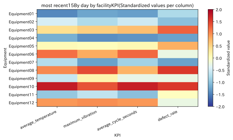

	average_temperature	maximum_vibration	average_cycle_seconds	defect_rate
Equipment
Equipment08	55.818	4.975	59.931	0.050
Equipment10	56.251	4.962	60.728	0.050
Equipment03	55.448	4.695	59.869	0.047
Equipment05	55.247	4.530	59.407	0.040
Equipment11	54.651	4.318	58.522	0.030

Reading the results

Equipment with overlapping red cells and multiple KPIs serves as entry points for narrowing down inspection candidates. However, standardized values change when the group changes. Alarm values based on equipment specifications, previous day differences, long-term trends, and measurement quality are checked, and causes are not automatically identified from graphs.

---

No.098: Numerical Error

Meaning in Practice

For sensor correction, accumulating minor differences, and simultaneous equations, even the same input may appear to have significantly different calculation results. If errors are mistaken for signs of failure, it can lead to unnecessary inspections or missed inspections.

Approach to Analysis and Modeling

The law of associative rule does not strictly hold with floating-point points. Also, if the number of conditions in $Ax=b$ is $\kappa(A)$, small input errors are amplified by the solution. Instead of explicitly creating the inverse matrix, use solve and specify the number of conditions and the residual $\lVert Ax-b\rVert/\lVert b\rVert$.

Check with Python

cancel_values = np.array([1e8, 1.0, -1e8], dtype=np.float32)
sum_forward = cancel_values.sum(dtype=np.float32)
sum_reordered = cancel_values[[0, 2, 1]].sum(dtype=np.float32)

A_good = np.array([[1.0, 0.2], [0.2, 1.0]])
A_bad = np.array([[1.0, 1.0], [1.0, 1.0 + 1e-10]])
b = np.array([2.0, 2.0 + 1e-10])
rows = []
for label, A in [("Stable calibration matrix", A_good), ("Almost duplicated proofreading matrices", A_bad)]:
    solution = np.linalg.solve(A, b)
    residual = np.linalg.norm(A @ solution - b) / np.linalg.norm(b)
    rows.append({"column": label, "Conditional number": np.linalg.cond(A), "relative residual": residual,
                 "solution1": solution[0], "solution2": solution[1]})
error_df = pd.DataFrame(rows)
print(f"float32Addition order: {sum_forward:.1f} And {sum_reordered:.1f}")
display(error_df.style.format({"Conditional number": "{:.2e}", "relative residual": "{:.2e}", "solution1": "{:.4f}", "solution2": "{:.4f}"}))

float32 addition order: 0.0 and 1.0

	column	Conditional number	relative residual	solution1	solution2
0	Stable calibration matrix	1.50e+00	1.57e-16	1.6667	1.6667
1	Almost duplicated proofreading matrices	4.00e+10	0.00e+00	1.0000	1.0000

Reading the results

In float32, the result changes only in the order of addition, and the nearly duplicated calibration matrix has a very large number of conditions. A small residual does not necessarily mean the solution is reliable. Units and scales are aligned, and float64, stable decomposition, recalibration, and regularization are considered, and the differences acceptable for business use are used as tests.

---

No.099: Benchmark

Meaning in Practice

Benchmarks create the basis for adopting GPUs and new libraries. Instead of using a single fastest value, it is repeated in a shape close to the actual data, comparing variation with the median and result matching.

Approach to Analysis and Modeling

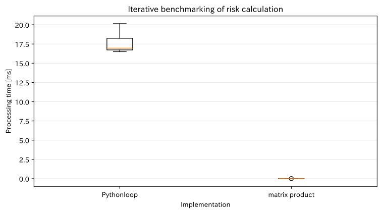
The initial preparation is separated, and candidates are alternately repeated under the same input and output conditions. Here, we measure the Python loop and matrix product of risk calculation multiple times, reporting median, quartile range, and 95th percentile. For processing that is too small, pay attention to the resolution of the measuring instruments.

Check with Python

def benchmark(func, *args, repeat=12):
    func(*args)  # warm-up
    samples = []
    for _ in range(repeat):
        start = time.perf_counter_ns()
        func(*args)
        samples.append((time.perf_counter_ns() - start) / 1e6)
    return np.array(samples)

bench = {"Pythonloop": benchmark(score_loop, Xz, w_fast),
         "matrix product": benchmark(score_vectorized, Xz, w_fast)}
bench_df = pd.DataFrame([
    {"Implementation": name, "median_ms": np.median(v), "IQR_ms": np.percentile(v, 75)-np.percentile(v, 25),
     "p95_ms": np.percentile(v, 95)} for name, v in bench.items()
])
display(bench_df.style.format({"median_ms": "{:.3f}", "IQR_ms": "{:.3f}", "p95_ms": "{:.3f}"}))

plt.boxplot([bench[k] for k in bench], tick_labels=list(bench))
plt.title("Iterative benchmarking of risk calculation")
plt.xlabel("Implementation")
plt.ylabel("Processing time [ms]")
plt.grid(True, axis="y", alpha=0.3)
plt.tight_layout()
plt.show()

	Implementation	median_ms	IQR_ms	p95_ms
0	Pythonloop	14.968	0.267	15.325
1	matrix product	0.005	0.001	0.009

Reading the results

In addition to the median, you can check stability from IQR and p95. These results are limited to the current device and data shape. Production candidates are evaluated using SLAs that include loading, preprocessing, computation, and output, while CI monitors trends for performance degradation. Numerical matching, memory, cost, and maintainability are also included in the adoption criteria.

---

No.100: The World of Matrix Computing

Meaning in Practice

The practical value of matrix calculation lies not in increasing the number of methods, but in organizing data into common representations and connecting calculation results to concrete actions. Finally, we integrate equipment risks from the latest data and create candidate inspections for the next day.

Approach to Analysis and Modeling

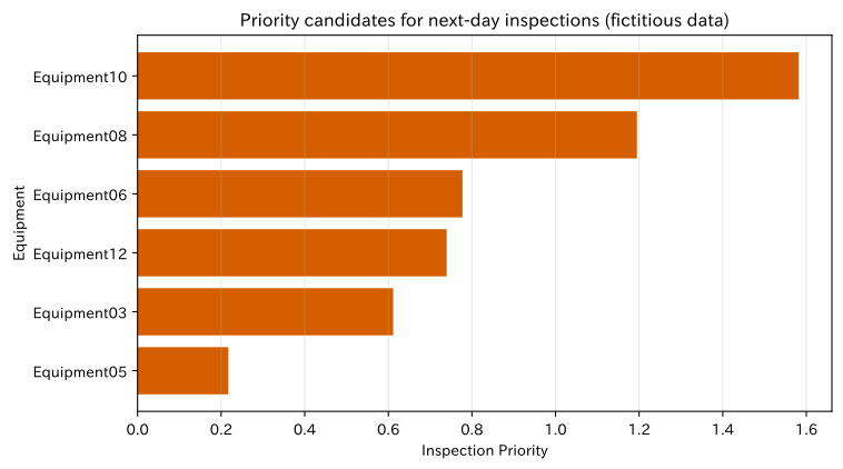
Define the priority of equipment $e$ as $P_e=0.45R_e+0.35V_e+0.20D_e$ from standardized average risk, maximum vibration, and failure rate. Weights are exemplary and are agreed upon with stakeholders as objective functions in practice, including stop loss, safety, quality impact, and inspection time. Top candidates are also paired with contribution KPIs.

Check with Python

risk_series = pd.Series(risk_fast, index=production_df.index, name="queue_risk")
decision = recent.assign(queue_risk=risk_series.loc[recent.index]).groupby("Equipment").agg(
    average_risk=("queue_risk", "mean"), maximum_vibration=("vibration_mm_s", "max"), defect_rate=("bad", "mean"),
    target_cycle=("bad", "size"),
)
decision_z = (decision[["average_risk", "maximum_vibration", "defect_rate"]] -
              decision[["average_risk", "maximum_vibration", "defect_rate"]].mean()) /              decision[["average_risk", "maximum_vibration", "defect_rate"]].std(ddof=0)
decision["Inspection Priority"] = decision_z @ np.array([0.45, 0.35, 0.20])
decision["Major ContributionsKPI"] = decision_z.idxmax(axis=1)
priority = decision.sort_values("Inspection Priority", ascending=False)
display(priority.head(5).style.format({"average_risk": "{:.3f}", "maximum_vibration": "{:.3f}", "defect_rate": "{:.2%}", "Inspection Priority": "{:.3f}"}))

top = priority.head(6).sort_values("Inspection Priority")
plt.barh(top.index, top["Inspection Priority"], color="#D55E00")
plt.title("Priority candidates for next-day inspections (fictitious data)")
plt.xlabel("Inspection Priority")
plt.ylabel("Equipment")
plt.grid(True, axis="x", alpha=0.3)
plt.tight_layout()
plt.show()

	average_risk	maximum_vibration	defect_rate	target_cycle	Inspection Priority	Major ContributionsKPI
Equipment
Equipment10	0.748	4.962	5.00%	300	1.582	average_risk
Equipment08	0.487	4.975	5.00%	300	1.195	defect_rate
Equipment06	0.585	4.782	2.67%	300	0.777	average_risk
Equipment12	0.518	4.842	2.67%	300	0.740	maximum_vibration
Equipment03	0.340	4.695	4.67%	300	0.612	defect_rate

Reading the results

Display top equipment and key contributing KPIs, allowing inspection teams to narrow down candidates to review. Priority is not the probability of failure, but a fictional relative score. During on-site implementation, mandatory safety inspections are prioritized under separate rules, inspection results are recorded, and weights and thresholds are updated. Matrix calculation is used not to replace decision-making but to help ensure consistency in the order of confirmations.

---

Practical Implications Seen Through Target Exercise

1. Select the board for the entire process: Not only the computational performance of CuPy and JAX, but also transfer, compilation, and post-processing are included.
2. Sharing table processing and matrix calculations: Narrow down to the necessary rows and columns in Polars, and clarify the boundaries for numerical calculations in NumPy and similar tools.
3. Improve algorithms first: After confirming vectorization and reducing unnecessary copies, consider GPU and parallelization.
4. Reproducibility is part of the deliverable.: Input fingerprints, parameters, environment, and verification results are stored in the notebook.
5. Measuring speed and accuracy simultaneously: Benchmarks include result concordance, margin of error, median, and variation.
6. Connecting Visualization to Action: Clarify inspection candidates, contributing KPIs, confirmation deadlines, and responsibilities.
7. Decisions that do not require advanced technology are also valuable.: If the data volume and SLA are small, CPU processing that is easy to maintain is more reasonable.

What is necessary for practical implementation

1. Define SLA and Decision Units

Set deadlines such as “until 7 a.m. every day” or “within 30 seconds after equipment shutdown,” and quantify target equipment, update frequency, acceptable delays, and concurrent users. Evaluation is based on whether decisions are made in time, not by acceleration rate.

2. Fix the correct answers, tolerance for error, and performance standards

Baseline implementations and representative data are stored, and KPIs, rankings, missing processing, and numerical tolerances are automatically inspected. The median and p95, peak memory, failure rate, and rerun time are accepted criteria.

3. Manage the execution environment and data

Records Python library drivers, random number seeds, input schemas, equipment ledgers, and model weights. When using a GPU, check driver compatibility and CPU fallback; for notebooks, check for full cell rerun.

4. Conduct small-scale operational verification

On a single line, you will try everything from presenting candidates, verifying the site, taking measures, to recording results. We evaluate missed items, unnecessary inspections, shortened time, and downtime losses, and estimate the computational resources and support systems for the entire factory deployment.

Conclusion

From No.091 to No.100, we used fictitious machining experience to verify CuPy’s GPU transfer estimates, pure functions and gradient validation leading to JAX, delayed aggregation with Polars, accelerated matrix computation, parallelization, notebook reproducibility, decision-making visualization, numerical errors, iterative benchmarking, and integration into inspection prioritization.

In manufacturing, choosing the fastest library is not important. Within the deadline, with permissible margins of error, produce reproducible results, demonstrate the basis and limitations, and guide on-site actions..

Consultations for Corporations

At Sukari Kobo, we support everything related to manufacturing’s processing, quality, and equipment data, including organizing data infrastructure, speeding up Python processing, evaluating the adoption of GPUs and parallel computations, standardizing notebooks, benchmark design, and visualizing inspection and quality judgments.

You can consult us about challenges such as “processing cannot keep up with all factory deployments,” “wanting to verify GPU implementation effects before investment,” “moving notebook analysis to reproducible operations,” and “how to verify numerical differences after speed improvements.”

📩 Contact Us: surikobo.co.jp/contact
Please feel free to consult us first.