100 Exercises / column / 100 Exercises in the Line

Learning predictive maintenance in manufacturing with Python | Practical applications of Transformer, GNN, and matrix decomposition

2020-03-10

Design the next inspection based on maintenance history and equipment network

Transformer, Embedded, GNN, Large Matrix Computation: 100 Exercises No.061–No.070

In manufacturing sites, data such as alarm order triggers, work records, and connections between equipment and parts is increasing, making it difficult to capture in tabular form alone. In this article, we use a fictional machining line as the subject, treating Capture historical context, find similar equipment and components, propagate risks from the network, and estimate the scale of computation. as a single decision story.

[!NOTE] This material is a notebook previously used by Surikoubo (or personally by the representative, Kazuyama), and has been reconstructed, edited, and published with the company’s permission.
All data listed is fictional and has no relation whatsoever to real companies, factories, or figures.

Introduction: Practical Challenges in Manufacturing Covered in This Article

In the fictional factory, alarms, inspections, and parts replacement histories are recorded for each piece of equipment. However, even with the same “vibration” alarm, the meaning changes depending on whether there was an overload before or after refueling. Additionally, newly installed equipment has few breakdowns, making it difficult to prioritize inspections based solely on individual data.

Therefore, the context of the time series, similarity of equipment and parts, and connections of equipment networks are represented in matrices, and the next equipment to be checked is narrowed down. The goal is not to string together AI terms, but to Converting maintenance decisions into considerations of stop losses and inspection man-hours.

Common situations on site

Threshold monitoring for single alarms cannot handle the order of occurrence or the meaning of simultaneous occurrences
There are significant fluctuations in the display of work records and significant differences in data volume between equipment
Knowledge from similar equipment has not been horizontally extended to newly installed facilities.
Overlooking the ripple effects caused by shared parts and process connections
Even if PoC works, expanding to all factories causes a sharp increase in memory and computation time

Why is this issue so difficult to judge?

History is not a “set of rows” but has an order, and the equipment network is not independent of each other. Furthermore, while embedding and deep learning scores are convenient, they cannot be operated if you ignore biased training data, unknown equipment, computational resources, and accountability.

In this article, we visualize the principle using small matrices. Instead of reproducing production implementations of Transformers or GNNs, we separate the core matrix operations of each method from the outputs and limits that maintenance personnel need to check.

Overview of Exercise covered this time

No.	Theme	Judgment in the manufacturing industry
061	Transformer	Which events in the history should be referenced to determine current risk?
062	embedding	Quantifying the similarity of equipment, parts, and alarms
063	matrix factorization	Summarize the history matrix into a few latent factors
064	Matrix Factorization	Unobserved equipment—supplementing component risks
065	LightGCN	Transmitting knowledge from connection relationships to similar equipment
066	Graph Neural Network	Consolidate connections and equipment features simultaneously
067	deep learning	Expressing nonlinear failure risks
068	automatic differentiation	Determining the update direction for each parameter from losses
069	GPU Computing	Estimating the scale needed to speed up matrix computation
070	Large-scale matrix computation	Expand to full factory scale with sparse queues

Preparing the Python environment

Dense matrix calculations are performed in NumPy, tables in pandas, sparse matrices in SciPy, and visualization in Matplotlib. It does not depend on external data or GPU-specific libraries. The random number generator is fixed at np.random.default_rng(61).

%matplotlib inline
%config InlineBackend.figure_format = 'svg'

import platform
import sys
import time

import japanize_matplotlib
import matplotlib
import matplotlib.pyplot as plt
import numpy as np
import pandas as pd
import scipy
from IPython.display import display
from scipy import sparse

rng = np.random.default_rng(61)
pd.set_option("display.precision", 4)

print("Python:", sys.version.split()[0])
print("OS:", platform.platform())
print("NumPy:", np.__version__)
print("pandas:", pd.__version__)
print("SciPy:", scipy.__version__)
print("Matplotlib:", matplotlib.__version__)

Python: 3.13.1
OS: macOS-26.3-arm64-arm-64bit-Mach-O
NumPy: 2.5.1
pandas: 3.0.3
SciPy: 1.18.0
Matplotlib: 3.11.0

Creation of Fictional Data

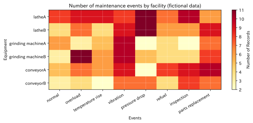
Fictional data is created for six pieces of equipment, eight types of maintenance events, and seven types of parts. Equipment has latent characteristics such as “rotary system,” “hydraulic system,” and “conveyor system,” and the usage trends of events and parts change accordingly.

In practice, the quality of analysis is determined by event dictionaries, equipment hierarchies, time granularity, and the distinction between ‘no record’ and ‘no occurrence.’ Here, we will limit ourselves to a scale that can foresee the underlying principles.

equipment = ["latheA", "latheB", "grinding machineA", "grinding machineB", "conveyorA", "conveyorB"]
events = ["normal", "overload", "temperature rise", "vibration", "pressure drop", "refuel", "inspection", "parts replacement"]
parts = ["spindle bearing", "whetstone", "hydraulic pump", "Seal", "conveyor belt", "Motor", "lubricating oil"]

# Row: Equipment, Column: Latent Characteristics (Rotational, Hydraulic, Conveying)
equipment_type = np.array([
    [1.0, 0.4, 0.1], [0.9, 0.5, 0.1], [1.0, 0.2, 0.1],
    [0.9, 0.3, 0.1], [0.2, 0.1, 1.0], [0.2, 0.2, 0.9],
])
event_affinity = np.array([
    [0.2, 0.2, 0.1], [0.8, 0.3, 0.4], [0.7, 0.4, 0.2], [1.0, 0.1, 0.2],
    [0.1, 1.0, 0.1], [0.4, 0.8, 0.3], [0.4, 0.4, 0.4], [0.8, 0.5, 0.7],
])
counts = rng.poisson(2 + 7 * (equipment_type @ event_affinity.T))
history_df = pd.DataFrame(counts, index=equipment, columns=events)

sequences = [
    ["normal", "overload", "temperature rise", "vibration", "inspection"],
    ["normal", "refuel", "normal", "overload", "temperature rise"],
    ["normal", "vibration", "vibration", "parts replacement", "normal"],
    ["normal", "temperature rise", "refuel", "normal", "inspection"],
    ["normal", "pressure drop", "overload", "inspection", "normal"],
    ["normal", "overload", "pressure drop", "temperature rise", "inspection"],
]
display(history_df)
display(pd.DataFrame(sequences, index=equipment, columns=[f"point in time{i}" for i in range(1, 6)]))

fig, ax = plt.subplots(figsize=(9, 4.2))
im = ax.imshow(history_df, cmap="YlOrRd", aspect="auto")
ax.set_title("Number of maintenance events by facility (fictional data)")
ax.set_xlabel("Events")
ax.set_ylabel("Equipment")
ax.set_xticks(range(len(events)), events, rotation=30, ha="right")
ax.set_yticks(range(len(equipment)), equipment)
ax.grid(True, color="white", linewidth=0.4, alpha=0.6)
fig.colorbar(im, ax=ax, label="Number of Records")
plt.tight_layout()
plt.show()

	normal	overload	temperature rise	vibration	pressure drop	refuel	inspection	parts replacement
latheA	8	9	9	8	11	7	10	6
latheB	4	7	4	9	11	6	6	9
grinding machineA	6	3	5	10	2	4	2	7
grinding machineB	3	11	6	10	5	4	4	8
conveyorA	5	7	6	9	2	8	9	10
conveyorB	3	4	2	7	7	4	8	7

	point in time1	point in time2	point in time3	point in time4	point in time5
latheA	normal	overload	temperature rise	vibration	inspection
latheB	normal	refuel	normal	overload	temperature rise
grinding machineA	normal	vibration	vibration	parts replacement	normal
grinding machineB	normal	temperature rise	refuel	normal	inspection
conveyorA	normal	pressure drop	overload	inspection	normal
conveyorB	normal	overload	pressure drop	temperature rise	inspection

svg

No.061：Transformer

Meaning in Practice

When determining the current state, Transformer indicates how many past records are referenced with Attention. Because it can handle alarm sequences and distant maintenance records, it is used for failure warnings, work log classification, and maintenance record summarization.

Approach to Analysis and Modeling

Create Query, Key, and Value from the representations at each point in time, and apply Scaled Dot-Product Attention

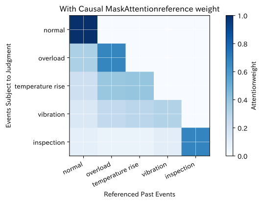
\operatorname{Attention}(Q,K,V)=\operatorname{softmax}\left(\frac{QK^\mathsf{T}}{\sqrt{d_k}}+M\right)V

Calculate it as follows. For forecasts without looking ahead, use mask $M$ . Here, we visualize where the most recent point refers to the past, and rather than claiming the performance of a trained model, we examine how it works.

Check with Python

event_to_id = {name: i for i, name in enumerate(events)}
d_model = 6
token_embedding = rng.normal(0, 0.7, size=(len(events), d_model))
position = np.arange(5)[:, None]
position_encoding = np.column_stack([
    np.sin(position[:, 0] / (10000 ** (2 * k / d_model))) if k % 2 == 0
    else np.cos(position[:, 0] / (10000 ** (2 * (k - 1) / d_model)))
    for k in range(d_model)
])

seq = sequences[0]
X_seq = token_embedding[[event_to_id[x] for x in seq]] + position_encoding
Q = K = V = X_seq
scores = Q @ K.T / np.sqrt(d_model)
causal_mask = np.triu(np.full_like(scores, -np.inf), k=1)
masked_scores = scores + causal_mask
weights = np.exp(masked_scores - np.max(masked_scores, axis=1, keepdims=True))
weights = weights / weights.sum(axis=1, keepdims=True)
context = weights @ V

display(pd.DataFrame(weights, index=[f"judgment:{x}" for x in seq], columns=[f"References:{x}" for x in seq]).style.format("{:.2f}"))
fig, ax = plt.subplots(figsize=(7.4, 4.4))
im = ax.imshow(weights, cmap="Blues", vmin=0, vmax=1)
ax.set_title("With Causal MaskAttentionreference weight")
ax.set_xlabel("Referenced Past Events")
ax.set_ylabel("Events Subject to Judgment")
ax.set_xticks(range(5), seq, rotation=25, ha="right")
ax.set_yticks(range(5), seq)
ax.grid(True, color="white", linewidth=0.4)
fig.colorbar(im, ax=ax, label="Attentionweight")
plt.tight_layout()
plt.show()

	References:normal	References:overload	References:temperature rise	References:vibration	References:inspection
judgment:normal	1.00	0.00	0.00	0.00	0.00
judgment:overload	0.33	0.67	0.00	0.00	0.00
judgment:temperature rise	0.21	0.39	0.40	0.00	0.00
judgment:vibration	0.14	0.26	0.28	0.31	0.00
judgment:inspection	0.09	0.07	0.06	0.10	0.67

svg

Reading the results

Since the upper triangle is 0, no future records are referenced at each point in time. The most recent contextual expression of “inspection” integrates past overloads, temperature rises, and vibrations with weighting. In practice, weights are not definitively judged as causal basis, but lead time before failure, missed rates, equipment-specific performance, and data leakage are verified.

No.062: Embedding

Meaning in Practice

Embedding converts facilities and events into small-dimensional vectors, allowing you to search for “objects with similar histories” by distance or dot product. It can be used to consolidate records with different notations, search for similar equipment for newly installed equipment, and suggest candidate maintenance items.

Approach to Analysis and Modeling

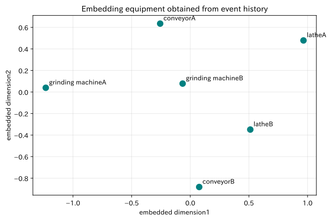
Equipment—standardize event queues and create equipment embedding $E=U_r\Sigma_r$ from SVD. cosine similarity

\operatorname{sim}(i,j)=\frac{\boldsymbol{e}_i^\mathsf{T}\boldsymbol{e}_j}{\lVert\boldsymbol{e}_i\rVert_2\lVert\boldsymbol{e}_j\rVert_2}

to measure how close the direction is. Since similarity does not imply causality or substitutability, cross-reconciling with equipment specifications is necessary.

Check with Python

H = np.log1p(history_df.to_numpy())
H_centered = H - H.mean(axis=0, keepdims=True)
U_h, s_h, Vt_h = np.linalg.svd(H_centered, full_matrices=False)
equipment_embedding = U_h[:, :2] * s_h[:2]
norms = np.linalg.norm(equipment_embedding, axis=1, keepdims=True)
cosine = (equipment_embedding @ equipment_embedding.T) / np.maximum(norms @ norms.T, 1e-12)

embedding_df = pd.DataFrame(equipment_embedding, index=equipment, columns=["embedding1", "embedding2"])
display(embedding_df.style.format("{:+.3f}"))
display(pd.DataFrame(cosine, index=equipment, columns=equipment).style.format("{:.2f}"))

fig, ax = plt.subplots(figsize=(7.2, 4.8))
ax.scatter(equipment_embedding[:, 0], equipment_embedding[:, 1], s=80, color="teal")
for i, name in enumerate(equipment):
    ax.annotate(name, equipment_embedding[i], xytext=(5, 5), textcoords="offset points")
ax.set_title("Embedding equipment obtained from event history")
ax.set_xlabel("embedded dimension1")
ax.set_ylabel("embedded dimension2")
ax.grid(True, alpha=0.3)
plt.tight_layout()
plt.show()

	embedding1	embedding2
latheA	+0.965	+0.479
latheB	+0.512	-0.349
grinding machineA	-1.232	+0.039
grinding machineB	-0.065	+0.078
conveyorA	-0.257	+0.635
conveyorB	+0.076	-0.882

	latheA	latheB	grinding machineA	grinding machineB	conveyorA	conveyorB
latheA	1.00	0.49	-0.88	-0.23	0.08	-0.37
latheB	0.49	1.00	-0.84	-0.96	-0.83	0.63
grinding machineA	-0.88	-0.84	1.00	0.66	0.40	-0.12
grinding machineB	-0.23	-0.96	0.66	1.00	0.95	-0.82
conveyorA	0.08	-0.83	0.40	0.95	1.00	-0.96
conveyorB	-0.37	0.63	-0.12	-0.82	-0.96	1.00

svg

Reading the results

Facilities of the same system are placed in the same direction, allowing for the creation of similar candidate patterns for historical patterns. Maintenance procedures for equipment that are close to the same area are not reused; instead, the type, load, operating time, and failure mode are checked. Embedding is the entry point for candidate search, requiring narrowing down using equipment ledgers and on-site knowledge.

No.063: Matrix Factorization

Meaning in Practice

Matrix decomposition summarizes the relationships between numerous equipment × events into a few latent factors such as “rotational systems” and “hydraulic systems.” It is effective for organizing monitoring KPIs, compressing data, removing noise, and understanding the characteristics of equipment groups.

Approach to Analysis and Modeling

and the upper $r$ components are decomposed by SVD into $H=U\Sigma V^\mathsf{T}$ ,

H_r=U_r\Sigma_rV_r^\mathsf{T}

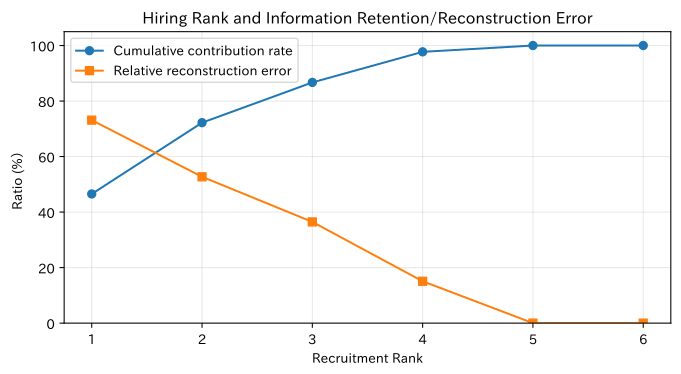
This approximates the situation. By examining the relative reconstruction error and cumulative contribution rate using the Frobenius norm, we compare simplification and information loss.

Check with Python

rank_rows = []
for rank in range(1, min(H.shape) + 1):
    H_rank = (U_h[:, :rank] * s_h[:rank]) @ Vt_h[:rank]
    rank_rows.append({
        "Rank": rank,
        "Cumulative contribution rate": np.sum(s_h[:rank] ** 2) / np.sum(s_h ** 2),
        "Relative reconstruction error": np.linalg.norm(H_centered - H_rank) / np.linalg.norm(H_centered),
    })
rank_df = pd.DataFrame(rank_rows)
display(rank_df.style.format({"Cumulative contribution rate": "{:.1%}", "Relative reconstruction error": "{:.1%}"}))

fig, ax = plt.subplots(figsize=(7.2, 4.0))
ax.plot(rank_df["Rank"], rank_df["Cumulative contribution rate"] * 100, marker="o", label="Cumulative contribution rate")
ax.plot(rank_df["Rank"], rank_df["Relative reconstruction error"] * 100, marker="s", label="Relative reconstruction error")
ax.set_title("Hiring Rank and Information Retention/Reconstruction Error")
ax.set_xlabel("Recruitment Rank")
ax.set_ylabel("Ratio (%）")
ax.set_ylim(0, 105)
ax.grid(True, alpha=0.3)
ax.legend()
plt.tight_layout()
plt.show()

	Rank	Cumulative contribution rate	Relative reconstruction error
0	1	46.5%	73.1%
1	2	72.2%	52.7%
2	3	86.7%	36.5%
3	4	97.7%	15.1%
4	5	100.0%	0.0%
5	6	100.0%	0.0%

svg

Reading the results

The higher the rank, the higher the information retention rate and the lower the reconstruction error. Even if the overview is captured with a few components, rare failures may appear in smaller components. Rankings are not determined solely by compression ratio; instead, recall rates and residual monitoring are used for each failure mode.

No.064：Matrix Factorization

Meaning in Practice

There are unobserved areas in equipment and parts combinations that are not necessarily low risk, just because there is no replacement record. Matrix Factorization learns latent factors from known relationships and supplements unobserved combinations as priority research candidates.

Approach to Analysis and Modeling

For the observation set $\Omega$ , find the equipment factor $P$ and the component factor $Q$ ,

\min_{P,Q}\sum_{(i,j)\in\Omega}(R_{ij}-\boldsymbol{p}_i^\mathsf{T}\boldsymbol{q}_j)^2 +\lambda(\lVert P\rVert_F^2+\lVert Q\rVert_F^2)

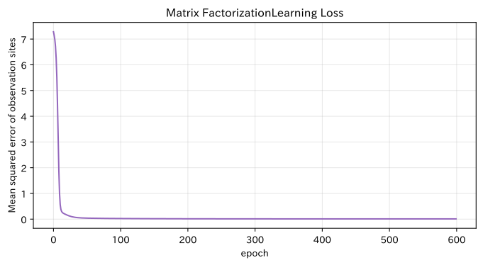
is minimized using stochastic gradient descent. It is important not to treat unobserved as zero and to separate it from evaluation.

Check with Python

part_factor = np.array([
    [1.0, 0.1, 0.1], [0.9, 0.1, 0.1], [0.2, 1.0, 0.1], [0.1, 0.9, 0.2],
    [0.1, 0.1, 1.0], [0.7, 0.2, 0.7], [0.4, 0.8, 0.3],
])
true_risk = 1 + 4 * (equipment_type @ part_factor.T) / 1.5
true_risk = np.clip(true_risk + rng.normal(0, 0.15, true_risk.shape), 1, 5)
observed = rng.random(true_risk.shape) < 0.68
R = np.where(observed, true_risk, np.nan)

k = 3
P = rng.normal(0, 0.3, size=(len(equipment), k))
Q = rng.normal(0, 0.3, size=(len(parts), k))
lr, reg = 0.025, 0.02
losses = []
obs_pairs = np.argwhere(observed)
for epoch in range(600):
    for i, j in obs_pairs[rng.permutation(len(obs_pairs))]:
        err = R[i, j] - P[i] @ Q[j]
        p_old = P[i].copy()
        P[i] += lr * (err * Q[j] - reg * P[i])
        Q[j] += lr * (err * p_old - reg * Q[j])
    pred = P @ Q.T
    losses.append(np.mean((R[observed] - pred[observed]) ** 2))

prediction = np.clip(P @ Q.T, 1, 5)
candidates = pd.DataFrame([
    {"Equipment": equipment[i], "Parts": parts[j], "Predicted Risk": prediction[i, j]}
    for i, j in np.argwhere(~observed)
]).sort_values("Predicted Risk", ascending=False)
display(candidates.head(8).style.format({"Predicted Risk": "{:.2f}"}))

fig, ax = plt.subplots(figsize=(7.2, 4.0))
ax.plot(losses, color="tab:purple")
ax.set_title("Matrix FactorizationLearning Loss")
ax.set_xlabel("epoch")
ax.set_ylabel("Mean squared error of observation sites")
ax.grid(True, alpha=0.3)
plt.tight_layout()
plt.show()

	Equipment	Parts	Predicted Risk
0	latheA	spindle bearing	3.66
2	latheB	whetstone	3.04
1	latheA	lubricating oil	2.89
3	latheB	hydraulic pump	2.43
4	latheB	Seal	2.31
6	conveyorA	lubricating oil	2.11
7	conveyorB	spindle bearing	1.71
5	grinding machineB	conveyor belt	1.33

svg

Reading the results

Predicted values are added to the unobserved equipment-parts combination, allowing you to rank candidates for additional inspections or ledger checks. However, learning errors based only on observed areas do not guarantee accuracy in unknown areas. We design tests based on chronological analysis, biases in ease of replacement, and masks for essential and non-equipped components.

No.065：LightGCN

Meaning in Practice

LightGCN propagates neighboring embeddings on a two-part equipment-component graph. By borrowing information from equipment that uses the same parts or parts used by similar equipment, you can suggest candidates even for subjects with little history.

Approach to Analysis and Modeling

Normalizing adjacency matrices without adding self-loops

\tilde{A}=D^{-1/2}AD^{-1/2},\qquad E^{(k+1)}=\tilde{A}E^{(k)}

and the mean of each layer as the final representation. Be careful of over-smoothing that causes the expression to be even out if you layer too many layers.

Check with Python

interaction = (true_risk >= 3.2).astype(float)
n_e, n_p = len(equipment), len(parts)
A = np.block([
    [np.zeros((n_e, n_e)), interaction],
    [interaction.T, np.zeros((n_p, n_p))],
])
degree = A.sum(axis=1)
D_inv_sqrt = np.diag(1 / np.sqrt(np.maximum(degree, 1)))
A_norm = D_inv_sqrt @ A @ D_inv_sqrt
E0 = rng.normal(0, 0.3, size=(n_e + n_p, 4))
layers = [E0]
for _ in range(3):
    layers.append(A_norm @ layers[-1])
E_light = np.mean(layers, axis=0)
light_scores = E_light[:n_e] @ E_light[n_e:].T

layer_change = [np.mean(np.linalg.norm(layers[i + 1] - layers[i], axis=1)) for i in range(3)]
display(pd.DataFrame(light_scores, index=equipment, columns=parts).style.format("{:+.2f}"))

fig, ax = plt.subplots(figsize=(7.2, 4.0))
ax.bar(["0→1layer", "1→2layer", "2→3layer"], layer_change, color="steelblue")
ax.set_title("LightGCNEmbedding changes by propagation layer")
ax.set_xlabel("propagation step")
ax.set_ylabel("Average change per node")
ax.grid(True, axis="y", alpha=0.3)
plt.tight_layout()
plt.show()

	spindle bearing	whetstone	hydraulic pump	Seal	conveyor belt	Motor	lubricating oil
latheA	+0.11	+0.09	-0.03	-0.01	+0.03	+0.06	+0.01
latheB	+0.05	+0.04	-0.02	-0.01	+0.00	+0.07	-0.01
grinding machineA	+0.11	+0.11	-0.03	+0.00	+0.03	-0.02	+0.04
grinding machineB	+0.09	+0.09	-0.03	+0.00	+0.06	+0.01	+0.02
conveyorA	+0.03	+0.05	-0.02	-0.02	+0.03	+0.07	+0.02
conveyorB	+0.01	+0.03	-0.01	-0.01	+0.07	+0.05	+0.00

svg

Reading the results

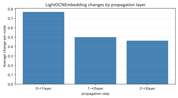
Not only does it involve direct relationships with components, but also information through equipment connecting to the same parts is included. As the layers progress, the amount of change decreases, and excessive propagation causes the differences between equipment to be lost. In practice, we verify the number of layers, definitions of negative instances, newly created nodes, and graph update frequency.

No.066：Graph Neural Network

Meaning in Practice

GNN aggregates not only connection relationships but also characteristics of each facility from nearby sources, such as operating rate, elapsed years, and number of abnormalities. It can be used for risk assessment that considers process relationships and shared parts networks.

Approach to Analysis and Modeling

Using the normalized adjacency matrix $\hat{A}$ with self-looping, the single-layer Graph Convolution

H^{(1)}=\operatorname{ReLU}(\hat{A}XW)

Let’s say so. $X$ is the equipment feature, and $W$ is the learning parameter. Here, we will compare only the effect of neighborhood aggregation with fixed weights.

Check with Python

# Equipment graph simplifying process order and shared parts
equipment_adj = np.array([
    [0, 1, 1, 0, 0, 0], [1, 0, 0, 1, 0, 0], [1, 0, 0, 1, 1, 0],
    [0, 1, 1, 0, 0, 1], [0, 0, 1, 0, 0, 1], [0, 0, 0, 1, 1, 0],
], dtype=float)
X_equipment = np.column_stack([
    np.array([0.82, 0.77, 0.91, 0.88, 0.70, 0.74]),  # Utilization rate
    np.array([8, 4, 11, 6, 5, 9]) / 12,              # Elapsed years (scaled)
    history_df[["vibration", "temperature rise", "pressure drop"]].sum(axis=1).to_numpy() / 40,
])
A_self = equipment_adj + np.eye(n_e)
D_self = np.diag(1 / np.sqrt(A_self.sum(axis=1)))
A_hat = D_self @ A_self @ D_self
W_gnn = np.array([[0.7, -0.3], [0.4, 0.8], [1.1, 0.5]])
H_gnn = np.maximum(0, A_hat @ X_equipment @ W_gnn)
local_only = np.maximum(0, X_equipment @ W_gnn)

gnn_df = pd.DataFrame({
    "local expression1": local_only[:, 0], "After neighborhood consolidation1": H_gnn[:, 0],
    "local expression2": local_only[:, 1], "After neighborhood consolidation2": H_gnn[:, 1],
}, index=equipment)
display(gnn_df.style.format("{:.3f}"))

fig, ax = plt.subplots(figsize=(8.0, 4.2))
x = np.arange(n_e)
ax.bar(x - 0.18, local_only[:, 0], width=0.36, label="Private facilities only")
ax.bar(x + 0.18, H_gnn[:, 0], width=0.36, label="After neighborhood consolidation")
ax.set_title("GNNNeighborhood consolidation of facility features")
ax.set_xlabel("Equipment")
ax.set_ylabel("Expression value (Index1dimension)")
ax.set_xticks(x, equipment)
ax.grid(True, axis="y", alpha=0.3)
ax.legend()
plt.tight_layout()
plt.show()

	local expression1	After neighborhood consolidation1	local expression2	After neighborhood consolidation2
latheA	1.611	1.406	0.637	0.519
latheB	1.332	1.383	0.336	0.439
grinding machineA	1.471	1.506	0.673	0.549
grinding machineB	1.394	1.464	0.399	0.532
conveyorA	1.124	1.219	0.336	0.499
conveyorB	1.258	1.196	0.578	0.420

svg

Reading the results

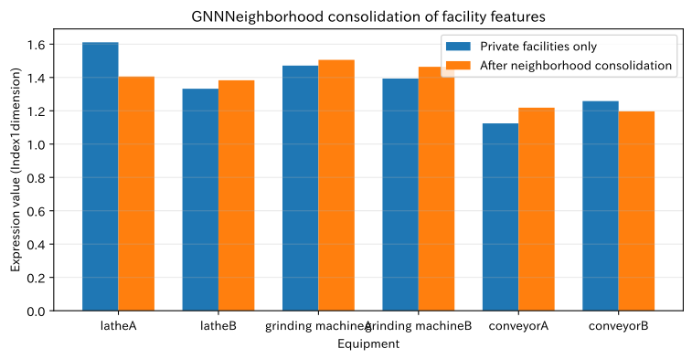
There is a difference between expressions that refer only to your own equipment and those that include connected equipment. While it is useful at sites where upstream equipment abnormalities affect downstream, its meaning changes depending on whether connections are undirected, time delays, and how flow is weighted. Agree on graph definitions with facility engineers to prevent false impact propagation.

No.067: Deep Learning

Meaning in Practice

Deep learning can learn nonlinear failure risks, such as combinations of temperature and load, which are difficult to represent with simple additions. It also serves as a foundation for integrating images, waveforms, and history.

Approach to Analysis and Modeling

Two-layer neural networks

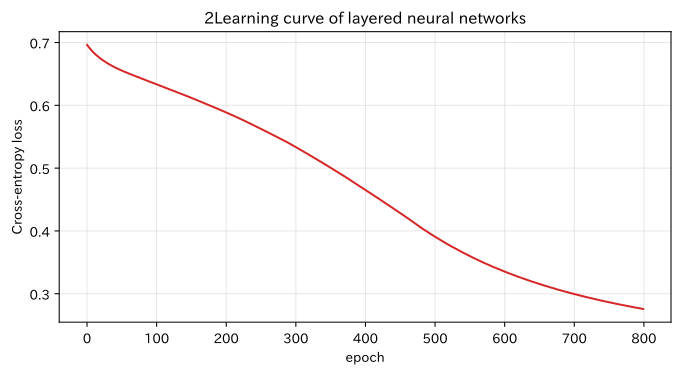
H=\operatorname{ReLU}(XW_1+b_1),\qquad \hat{y}=\sigma(HW_2+b_2)

Let’s say so. Here, we create binary labels from imaginary equipment conditions and learn using the gradient descent method. Not only training accuracy but also external verification by equipment and duration is necessary.

Check with Python

n_samples = 500
X_dl = rng.normal(size=(n_samples, 3))
nonlinear_risk = 1.3 * X_dl[:, 0] * X_dl[:, 1] + 0.9 * X_dl[:, 2] ** 2 - 0.5
y_dl = (nonlinear_risk + rng.normal(0, 0.35, n_samples) > 0).astype(float)[:, None]
split = 400
mean_dl, std_dl = X_dl[:split].mean(axis=0), X_dl[:split].std(axis=0)
X_dl = (X_dl - mean_dl) / std_dl

W1 = rng.normal(0, 0.3, size=(3, 8)); b1 = np.zeros((1, 8))
W2 = rng.normal(0, 0.3, size=(8, 1)); b2 = np.zeros((1, 1))
lr_dl = 0.08
dl_losses = []
for epoch in range(800):
    Xb, yb = X_dl[:split], y_dl[:split]
    z1 = Xb @ W1 + b1
    h = np.maximum(0, z1)
    logits = h @ W2 + b2
    prob = 1 / (1 + np.exp(-np.clip(logits, -30, 30)))
    loss = -np.mean(yb * np.log(prob + 1e-9) + (1 - yb) * np.log(1 - prob + 1e-9))
    dl_losses.append(loss)
    dlogits = (prob - yb) / split
    dW2, db2 = h.T @ dlogits, dlogits.sum(axis=0, keepdims=True)
    dh = dlogits @ W2.T
    dz1 = dh * (z1 > 0)
    dW1, db1 = Xb.T @ dz1, dz1.sum(axis=0, keepdims=True)
    W1 -= lr_dl * dW1; b1 -= lr_dl * db1
    W2 -= lr_dl * dW2; b2 -= lr_dl * db2

def mlp_predict(X):
    hidden = np.maximum(0, X @ W1 + b1)
    return 1 / (1 + np.exp(-np.clip(hidden @ W2 + b2, -30, 30)))

train_acc = np.mean((mlp_predict(X_dl[:split]) >= 0.5) == y_dl[:split])
test_acc = np.mean((mlp_predict(X_dl[split:]) >= 0.5) == y_dl[split:])
display(pd.DataFrame({"Classification": ["Learning", "Reception"], "Accuracy rate": [train_acc, test_acc]}).style.format({"Accuracy rate": "{:.1%}"}))

fig, ax = plt.subplots(figsize=(7.2, 4.0))
ax.plot(dl_losses, color="tab:red")
ax.set_title("2Learning curve of layered neural networks")
ax.set_xlabel("epoch")
ax.set_ylabel("Cross-entropy loss")
ax.grid(True, alpha=0.3)
plt.tight_layout()
plt.show()

	Classification	Accuracy rate
0	Learning	90.0%
1	Reception	89.0%

svg

Reading the results

Losses are reduced, and a certain classification performance is achieved with nonlinear relationships in fictional data. However, accuracy alone cannot assess the cost of missed or false stops for rare failures. Check accuracy, recall, calibration, and lead time, and adopt it when improvements over simple models justify operational costs.

No.068: Automatic Differentiation

Meaning in Practice

Because deep learning has many parameters, it cannot manually calculate how losses affect each parameter. Automatic differentiation applies the chain law to computational graphs to determine gradients accurately and efficiently.

Approach to Analysis and Modeling

Even with simple predictions $\hat{y}=wx+b$ loss $L=(\hat{y}-y)^2$ , by the chain law,

\frac{\partial L}{\partial w}=2(\hat{y}-y)x,\qquad \frac{\partial L}{\partial b}=2(\hat{y}-y)

That’s right. Implement a small inverse automatic differential class and match it with finite differences. In production, we use a well-validated framework.

Check with Python

class Value:
    def __init__(self, data, parents=(), grads=()):
        self.data = float(data)
        self.grad = 0.0
        self.parents = parents
        self.grads = grads
    def __add__(self, other):
        other = other if isinstance(other, Value) else Value(other)
        return Value(self.data + other.data, (self, other), (1.0, 1.0))
    __radd__ = __add__
    def __mul__(self, other):
        other = other if isinstance(other, Value) else Value(other)
        return Value(self.data * other.data, (self, other), (other.data, self.data))
    __rmul__ = __mul__
    def __neg__(self):
        return self * -1
    def __sub__(self, other):
        return self + (-other)
    def __pow__(self, power):
        return Value(self.data ** power, (self,), (power * self.data ** (power - 1),))
    def backward(self):
        topo, seen = [], set()
        def build(v):
            if id(v) not in seen:
                seen.add(id(v))
                for p in v.parents: build(p)
                topo.append(v)
        build(self)
        self.grad = 1.0
        for v in reversed(topo):
            for p, local_grad in zip(v.parents, v.grads):
                p.grad += v.grad * local_grad

x_ad, y_ad = 1.7, 4.2
w_ad, b_ad = Value(1.1), Value(0.3)
loss_ad = (w_ad * x_ad + b_ad - y_ad) ** 2
loss_ad.backward()

def scalar_loss(w, b):
    return (w * x_ad + b - y_ad) ** 2

eps = 1e-6
fd_w = (scalar_loss(1.1 + eps, 0.3) - scalar_loss(1.1 - eps, 0.3)) / (2 * eps)
fd_b = (scalar_loss(1.1, 0.3 + eps) - scalar_loss(1.1, 0.3 - eps)) / (2 * eps)
grad_df = pd.DataFrame({
    "Parameter": ["w", "b"], "automatic differentiation": [w_ad.grad, b_ad.grad],
    "finite difference": [fd_w, fd_b], "absolute difference": [abs(w_ad.grad - fd_w), abs(b_ad.grad - fd_b)],
})
display(grad_df.style.format({"automatic differentiation": "{:.6f}", "finite difference": "{:.6f}", "absolute difference": "{:.2e}"}))

fig, ax = plt.subplots(figsize=(7.2, 4.0))
ax.bar(np.arange(2) - 0.17, grad_df["automatic differentiation"], width=0.34, label="automatic differentiation")
ax.bar(np.arange(2) + 0.17, grad_df["finite difference"], width=0.34, label="finite difference")
ax.set_title("Gradient Matching Using Automatic Differentiation and Finite Difference")
ax.set_xlabel("Parameter")
ax.set_ylabel("Loss gradient")
ax.set_xticks(range(2), grad_df["Parameter"])
ax.grid(True, axis="y", alpha=0.3)
ax.legend()
plt.tight_layout()
plt.show()

	Parameter	automatic differentiation	finite difference	absolute difference
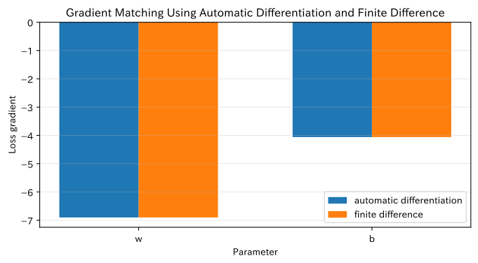
0	w	-6.902000	-6.902000	4.69e-10
1	b	-4.060000	-4.060000	2.50e-10

svg

Reading the results

The gradient of automatic differentiation matches the finite difference and the range of numerical error. In practice, gradient checks are performed using typical small-scale inputs to monitor implementation errors such as NaN, gradient loss and explosion, and loss. The ability to calculate gradients and the objective function correctly representing site losses are two separate things.

No.069: GPU Computing

Meaning in Practice

GPUs can perform numerous multiply-sum operations in parallel, accelerating deep learning and large-scale embedded computations. On the other hand, small table data is dominated by transfer and boot overhead, and sometimes the CPU is sufficient.

Approach to Analysis and Modeling

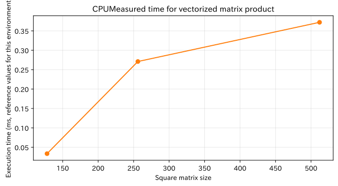
The matrix product of $m\times k$ and $k\times n$ generally requires $2mkn$ FLOP. The required memory is estimated including input, output, mid-range, and gradient. Here, without requiring a GPU, we calculate the computational load and minimum array memory for each matrix size, and also check the time for vectorized CPU computation.

Check with Python

sizes = [128, 512, 1024, 2048, 4096]
gpu_plan = pd.DataFrame({
    "Square matrix size": sizes,
    "Matrix product complexity_GFLOP": [2 * n**3 / 1e9 for n in sizes],
    "3Minimum Array Memory_GB_float32": [3 * n**2 * 4 / 1e9 for n in sizes],
    "3Minimum Array Memory_GB_float64": [3 * n**2 * 8 / 1e9 for n in sizes],
})
display(gpu_plan.style.format({
    "Matrix product complexity_GFLOP": "{:.2f}",
    "3Minimum Array Memory_GB_float32": "{:.3f}",
    "3Minimum Array Memory_GB_float64": "{:.3f}",
}))

bench_sizes = [128, 256, 512]
bench_times = []
for n in bench_sizes:
    a = rng.normal(size=(n, n)).astype(np.float32)
    b = rng.normal(size=(n, n)).astype(np.float32)
    start = time.perf_counter()
    _ = a @ b
    bench_times.append(time.perf_counter() - start)

fig, ax = plt.subplots(figsize=(7.2, 4.0))
ax.plot(bench_sizes, np.array(bench_times) * 1000, marker="o", color="tab:orange")
ax.set_title("CPUMeasured time for vectorized matrix product")
ax.set_xlabel("Square matrix size")
ax.set_ylabel("Execution time (ms, reference values for this environment)")
ax.grid(True, alpha=0.3)
plt.tight_layout()
plt.show()

	Square matrix size	Matrix product complexity_GFLOP	3Minimum Array Memory_GB_float32	3Minimum Array Memory_GB_float64
0	128	0.00	0.000	0.000
1	512	0.27	0.003	0.006
2	1024	2.15	0.013	0.025
3	2048	17.18	0.050	0.101
4	4096	137.44	0.201	0.403

svg

Reading the results

When the matrix size doubles, the computational load increases about eightfold, making it a candidate for GPUs at scale. However, the memory in the table is minimal, and during training, gradients, optimized states, and temporary areas are added. Using actual machine data, we measure end-to-end time including preprocessing, transfer, training, and inference, and make decisions on implementation based on delivery time, cost, and power consumption.

No.070: Large-Scale Matrix Computation

Meaning in Practice

The entire factory’s equipment—parts, equipment—event queues are mostly zero. If you keep it as a dense matrix, memory is used even where there is no data, unnecessarily increasing the computational scale. Sparse matrices only preserve relationships that actually exist.

Approach to Analysis and Modeling

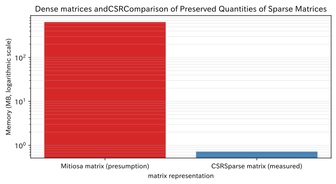
If the nonzero number in the $m\times n$ matrix is $\operatorname{nnz}$ , the amount stored in the dense matrix is $O(mn)$ , and the CSR format is approximately $O(\operatorname{nnz}+m)$ . The matrix vector product can also be calculated centered on nonzero elements. Choose the format based on sparseness, access patterns, and update frequency.

Check with Python

n_rows, n_cols, density = 20_000, 8_000, 0.0005
large_sparse = sparse.random(
    n_rows, n_cols, density=density, format="csr", dtype=np.float32, random_state=61,
)
vector = rng.normal(size=n_cols).astype(np.float32)
start = time.perf_counter()
result_sparse = large_sparse @ vector
sparse_time = time.perf_counter() - start

dense_bytes = n_rows * n_cols * np.dtype(np.float32).itemsize
csr_bytes = large_sparse.data.nbytes + large_sparse.indices.nbytes + large_sparse.indptr.nbytes
storage_df = pd.DataFrame({
    "Performance": ["Mitiosa matrix (presumption)", "CSRSparse matrix (measured)"],
    "Memory_MB": [dense_bytes / 1e6, csr_bytes / 1e6],
    "nonzero element count": [n_rows * n_cols, large_sparse.nnz],
})
display(storage_df.style.format({"Memory_MB": "{:,.2f}", "nonzero element count": "{:,.0f}"}))
print("Sparse matrix vector product:", f"{sparse_time * 1000:.2f} ms", "/ Output Shape:", result_sparse.shape)

fig, ax = plt.subplots(figsize=(7.2, 4.0))
ax.bar(storage_df["Performance"], storage_df["Memory_MB"], color=["tab:red", "steelblue"])
ax.set_yscale("log")
ax.set_title("Dense matrices andCSRComparison of Preserved Quantities of Sparse Matrices")
ax.set_xlabel("matrix representation")
ax.set_ylabel("Memory (MB, logarithmic scale)")
ax.grid(True, axis="y", which="both", alpha=0.3)
plt.tight_layout()
plt.show()

	Performance	Memory_MB	nonzero element count
0	Mitiosa matrix (presumption)	640.00	160,000,000
1	CSRSparse matrix (measured)	0.72	80,000

Sparse matrix vector product: 0.33 ms / Output shape: (20000,)

svg

Reading the results

For a matrix with only 0.05% value, the CSR format can hold much less memory than a dense matrix. For full-factory deployment, in addition to sparse matrixing, split processing, mini-batches, approximate search, incremental updates, and monitoring period limits are combined. The design includes not only execution time but also recalculation time, failure recovery, and data update consistency.

Practical Implications Seen Through Target Exercise

History includes order and context: Transformer’s Attention allows you to handle combinations of events that are not visible with a single alarm.
Embedding helps with candidate search.: You can quantify the similarity of equipment and parts, but specification verification and causal verification are required separately.
Unobserved is not zero: Matrix Factorization distinguishes between no records and no risk.
Network definitions determine the meaning of the model: LightGCN and GNN agree with the site on connection direction, weight, and time delay.
The more advanced the model, the more important it is to compare it with the reference model: Determine whether improving accuracy justifies the costs of explanation, operation, and calculation.
Computational resources are part of model design: Choose GPU, sparse matrix, and partitioning method based on data scale and update deadline.

What is necessary for practical implementation

1. Define the unit of judgment and the correct answer

Decide on the forecast targets and time window, such as “shutdown within 24 hours,” “parts replacement within 7 days,” and “inspection at the next scheduled maintenance.” Distinguish between alarms, work instructions, replacements, and cause confirmation, and record labels that may be biased toward on-site judgments.

2. Manage data and graphs

Manage equipment IDs, part IDs, event dictionaries, schedules, and equipment configuration versions. Reflect equipment expansions and process changes in the graph to monitor future information incorporation, record omissions, and changes in maintenance policies.

3. Verify step by step

Based on simple rules and regression criteria, evaluations are conducted by equipment and period, and recall rates by failure mode, false alarms, and lead times are compared. Attention and embedded visualization are used as explanatory aids and distinguished from causal explanations.

4. Design Operations, Calculation, and Responsibility Boundaries

We procedurally decide who identifies candidates, what additional measures are taken, and decisions to stop, continue, or follow-up are made. This includes retraining cycles, processing deadlines, GPU costs, alternative rules in case of failures, and version management of models and data.

Conclusion

From No.061 to No.070, we used fictional equipment history as the subject, examining Transformer attention, embedding, matrix factorization, Matrix Factorization, LightGCN, GNN, deep learning, automatic differentiation, GPU computation, and large-scale calculations using sparse matrices.

The key to leveraging these in manufacturing is not simply complicating the model. Accurately represent history, equipment configuration, and site losses, and connect them to operations from candidate proposal to confirmation and action..

Consultations for Corporations

At Surikoubo, we support everything from data organization to PoC, evaluation design, and on-site operations for maintenance history analysis, equipment and component network analysis, anomaly detection, predictive maintenance, recommendation and graph machine learning, and large-scale matrix calculations in manufacturing.

You can consult us about issues such as “wanting to connect alarm history to maintenance decisions,” “wanting to expand knowledge from similar equipment,” “verifying the validity of using GNNs and Transformers from reference models,” or “reviewing the computing infrastructure for full-factory deployment.”

📩 Contact Us: surikobo.co.jp/contact
Please feel free to consult us first.

Learning predictive maintenance in manufacturing with Python | Practical applications of Transformer, GNN, and matrix decomposition

Design the next inspection based on maintenance history and equipment network

Transformer, Embedded, GNN, Large Matrix Computation: 100 Exercises No.061–No.070

Introduction: Practical Challenges in Manufacturing Covered in This Article

Common situations on site

Why is this issue so difficult to judge?

Overview of Exercise covered this time

Preparing the Python environment

Creation of Fictional Data

No.061：Transformer

Meaning in Practice

Approach to Analysis and Modeling

Check with Python

Reading the results

No.062: Embedding

Meaning in Practice

Approach to Analysis and Modeling

Check with Python

Reading the results

No.063: Matrix Factorization

Meaning in Practice

Approach to Analysis and Modeling

Check with Python

Reading the results

No.064：Matrix Factorization

Meaning in Practice

Approach to Analysis and Modeling

Check with Python

Reading the results

No.065：LightGCN

Meaning in Practice

Approach to Analysis and Modeling

Check with Python

Reading the results

No.066：Graph Neural Network

Meaning in Practice

Approach to Analysis and Modeling

Check with Python

Reading the results

No.067: Deep Learning

Meaning in Practice

Approach to Analysis and Modeling

Check with Python

Reading the results

No.068: Automatic Differentiation

Meaning in Practice

Approach to Analysis and Modeling

Check with Python

Reading the results

No.069: GPU Computing

Meaning in Practice

Approach to Analysis and Modeling

Check with Python

Reading the results

No.070: Large-Scale Matrix Computation

Meaning in Practice

Approach to Analysis and Modeling

Check with Python

Reading the results

Practical Implications Seen Through Target Exercise

What is necessary for practical implementation

1. Define the unit of judgment and the correct answer

2. Manage data and graphs

3. Verify step by step

4. Design Operations, Calculation, and Responsibility Boundaries

Conclusion

Consultations for Corporations

Related Posts

Introduction to Python Acceleration in Manufacturing | CuPy, JAX, Polars, and Practical Matrix Computation

Integrating Quality, Demand, and Production Planning in Manufacturing with Python | Learning Matrix Analysis in Practice

Factory Simulation Implemented with Python | Decision-Making for Inventory, Queues, and Production Planning

Learning Manufacturing Quality Forecasting with Python | Introduction to Ridge, Logistic Regression, and Attention

Introduction to Process Network Analysis in Manufacturing | Learning PCA, PageRank, and GCN with Python