100 Exercises / column / 100 Exercises in the Line

Factory Simulation Implemented with Python | Decision-Making for Inventory, Queues, and Production Planning

2020-03-11

Designing processing lines resistant to fluctuations

State transition, inventory, queues, factory simulation: 100 Exercises No.071–No.080

On the manufacturing floor, equipment deterioration, demand fluctuations, waiting in the process, and stockouts all affect each other. In this article, we use a fictional precision parts line as a subject, treating The condition is represented as a matrix, individual models are combined, and improvement proposals are shared across the entire factory.KPICompare by as a single decision story.

[!NOTE] This material is a notebook previously used by Surikoubo (or personally by the representative, Kazuyama), and has been reconstructed, edited, and published with the company’s permission.
All data listed is fictional and has no relation whatsoever to real companies, factories, or figures.

Introduction: Practical Challenges in Manufacturing Covered in This Article

In a fictional factory, precision parts are produced through three processes: turning, grinding, and inspection. Increasing input volume in response to demand waves raises work-in-progress and waiting times, while shrinking inventory leads to more stockouts. The more equipment operates, the more deterioration it becomes, and sudden shutdowns can spread to subsequent processes.

Here, state transition matrices, inventory models, production planning, queues, Markov models, discrete event simulation, Monte Carlo method, digital twins, and optimization are used step by step. The goal is not to predict a precise future, but to Options for increasing staff, inventory, maintenance, and capital investment are the same.KPIComparing.

Common situations on site

You can see the operating rate of each facility, but it’s unclear how deterioration will accumulate into the following week and beyond.
Safety stock is determined based on experience, with no comparison between stock-out costs and storage costs
Monthly production schedules and daily waiting times and downtime are managed separately
Assess capability solely by average cycle time and overlook stagnation caused by variation.
Evaluation of improvement proposals based on a single assumption and failure to handle uncertainties in demand, failures, and machining time
Simulation results are not matched with field performance and are not used for decision-making

Why is this issue so difficult to judge?

A manufacturing line is a dynamic system where the state at one point affects the next. Even if the average values are the same, processes with large variation tend to have longer wait times, and speeding up local processes may not lead to increased shipments across the entire factory. Furthermore, demand, equipment failures, and repair times are probabilistic.

Refining the model in detail doesn’t necessarily bring you closer to reality. It is important to clearly state the basis for input values, model boundaries, KPI definitions, and comparison criteria, starting with simple calculations and adding only the necessary complexity. In this article, we represent the same fictional line in multiple resolutions, distinguishing the roles and limitations of each model.

Overview of Exercise covered this time

No.	Theme	Judgment in the manufacturing industry
071	State transition matrix	How will equipment deterioration and failure be distributed in the future?
072	Stock Model	How to set order points and safety stock
073	Production plan	What and how many to make within the capability constraints
074	queue	Is it necessary to increase staff and enhance capacity in inspection processes?
075	Markov Model	Comparing long-term operation and shutdown rates and conservation effects
076	Discrete Event Simulation	Recreate arrival, processing, and breakdowns as chronological events.
077	Monte Carlo method	Evaluating the probability of profit and delivery achievement, including uncertainties.
078	Digital twin	Calibration models based on performance and monitoring variances
079	Optimization	Where to allocate the limited improvement budget
080	Factory Simulation	Integrate individual initiatives and compare them against overall KPIs

Preparing the Python environment

Matrix and random number calculations are performed in NumPy, tables in pandas, optimization in SciPy, and visualization in Matplotlib. It does not rely on external data or dedicated simulation products. The random number generator is fixed at np.random.default_rng(71), and for policy comparisons, the seed is passed for each function so that the same random number series can be used.

%matplotlib inline
%config InlineBackend.figure_format = 'svg'

import heapq
import math
import platform
import sys
from itertools import combinations

import japanize_matplotlib
import matplotlib
import matplotlib.pyplot as plt
import numpy as np
import pandas as pd
import scipy
from IPython.display import display
from scipy.optimize import linprog

rng = np.random.default_rng(71)
pd.set_option("display.precision", 3)

print("Python:", sys.version.split()[0])
print("OS:", platform.platform())
print("NumPy:", np.__version__)
print("pandas:", pd.__version__)
print("SciPy:", scipy.__version__)
print("Matplotlib:", matplotlib.__version__)

Python: 3.13.1
OS: macOS-26.3-arm64-arm-64bit-Mach-O
NumPy: 2.5.1
pandas: 3.0.3
SciPy: 1.18.0
Matplotlib: 3.11.0

Creation of Fictional Data

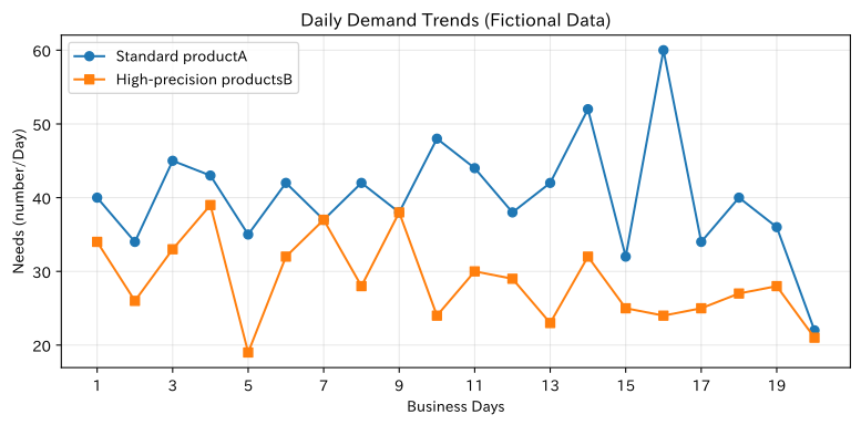
The line for turning and inspecting two products (Standard A and High-Precision B ) is conducted. Generate 20 business days’ worth of demand and performance cycle time. Demand varies by day of the week, and processing time is adjusted with long variations on the right hem.

In practice, you first define whether to include setup and breaks in stop times, whether to record machining start or completion, and how to handle reprocessing due to defects. Here, to help you understand the relationships between each model, we will unify the units as “pieces,” “minutes,” and “business days.”

products = ["Standard productA", "High-precision productsB"]
processes = ["turning", "grinding", "Examination"]
days = np.arange(1, 21)

base_demand = np.array([42, 27])
weekday_factor = np.array([1.08, 0.96, 1.02, 1.12, 0.82])
demand = np.vstack([
    rng.poisson(base_demand * weekday_factor[(d - 1) % 5]) for d in days
])
demand_df = pd.DataFrame(demand, index=[f"Day {d:02d}" for d in days], columns=products)

# Row: project, column: product. Standard cycle time (minutes/unit)
cycle_minutes = pd.DataFrame(
    [[6.0, 8.0], [7.5, 10.0], [4.0, 6.5]], index=processes, columns=products
)
observed_cycle = {
    p: rng.lognormal(np.log(cycle_minutes.loc[p].mean()) - 0.5 * 0.18**2, 0.18, 160)
    for p in processes
}

display(demand_df.head())
display(cycle_minutes)
fig, ax = plt.subplots(figsize=(8.2, 4.1))
ax.plot(days, demand[:, 0], marker="o", label=products[0])
ax.plot(days, demand[:, 1], marker="s", label=products[1])
ax.set_title("Daily Demand Trends (Fictional Data)")
ax.set_xlabel("Business Days")
ax.set_ylabel("Needs (number/Day)")
ax.set_xticks(days[::2])
ax.grid(True, alpha=0.3)
ax.legend()
plt.tight_layout()
plt.show()

	Standard productA	High-precision productsB
Day 01	40	34
Day 02	34	26
Day 03	45	33
Day 04	43	39
Day 05	35	19

	Standard productA	High-precision productsB
turning	6.0	8.0
grinding	7.5	10.0
Examination	4.0	6.5

svg

No.071: State Transition Matrix

Meaning in Practice

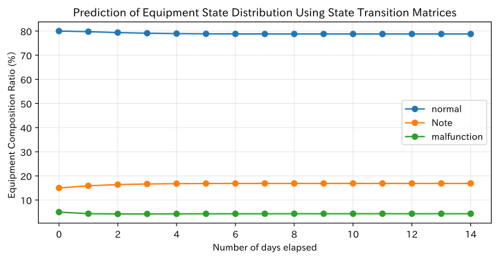
By dividing equipment status into “normal, cautionary, and faulty,” and representing the probability of moving from today’s status to tomorrow’s status as a matrix, you can anticipate the number of units to be inspected and the number of spare machines needed. Rather than determining the failure date of individual equipment, it is suitable for predicting the state composition of equipment groups.

Approach to Analysis and Modeling

If we set the state distribution as a row vector $\boldsymbol{p}_t$ and the transition matrix as $P$ , after $k$ days,

\boldsymbol{p}_{t+k}=\boldsymbol{p}_tP^k, \qquad P_{ij}=\Pr(S_{t+1}=j\mid S_t=i), \qquad \sum_jP_{ij}=1

to find it. Make sure the sum of the row is 1 and the probability is non-negative. When estimating based on actual results, it is important not to unconditionally mix periods when equipment models, load ranges, or maintenance policies have changed.

Check with Python

states = ["normal", "Note", "malfunction"]
P = np.array([
    [0.90, 0.09, 0.01],
    [0.30, 0.58, 0.12],
    [0.65, 0.00, 0.35],
])
p0 = np.array([0.80, 0.15, 0.05])
state_path = np.vstack([p0 @ np.linalg.matrix_power(P, k) for k in range(15)])
state_df = pd.DataFrame(state_path, index=np.arange(15), columns=states)

display(pd.DataFrame(P, index=[f"Now:{s}" for s in states], columns=[f"The next day:{s}" for s in states]))
display(state_df.iloc[[0, 1, 3, 7, 14]].style.format("{:.1%}"))
assert np.allclose(P.sum(axis=1), 1)

fig, ax = plt.subplots(figsize=(7.6, 4.0))
for state in states:
    ax.plot(state_df.index, state_df[state] * 100, marker="o", label=state)
ax.set_title("Prediction of Equipment State Distribution Using State Transition Matrices")
ax.set_xlabel("Number of days elapsed")
ax.set_ylabel("Equipment Composition Ratio (%）")
ax.grid(True, alpha=0.3)
ax.legend()
plt.tight_layout()
plt.show()

	The next day:normal	The next day:Note	The next day:malfunction
Now:normal	0.90	0.09	0.01
Now:Note	0.30	0.58	0.12
Now:malfunction	0.65	0.00	0.35

	normal	Note	malfunction
0	80.0%	15.0%	5.0%
1	79.8%	15.9%	4.3%
3	79.1%	16.7%	4.2%
7	78.8%	16.9%	4.3%
14	78.8%	16.9%	4.3%

svg

Reading the results

From the composition ratio on the first day, the attention to malfunction states approach a certain ratio over time. For example, if you have 20 units of equipment, you can estimate the expected number of units repaired by multiplying the predicted failure ratio by 20. However, the expected value does not necessarily mean the number of units will be the same. We check the number of transitions per day, differences by model, and initial failures after repairs, and operate with estimated errors in transition probabilities.

No.072: Stock Model

Meaning in Practice

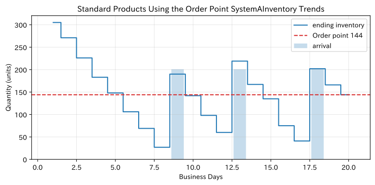
While inventory prevents stockouts, it also leads to storage costs, obsolescence, and financial constraints. In the order-point method, inventory positions are replenished when they fall below thresholds, absorbing demand fluctuations and procurement lead times.

Approach to Analysis and Modeling

Let the average daily demand be $\mu_d$ , standard deviation $\sigma_d$ , lead time $L$ days, and safety factor $z$ , then the order point assuming independent and identical distribution is

R=\mu_dL+z\sigma_d\sqrt{L}

That’s right. The first half is average demand during lead time, and the second half is safety stock. In practice, this includes weekday variability, demand correlation, lead time fluctuations itself, order lots, and outstanding balances.

Check with Python

daily_a = demand_df["Standard productA"].to_numpy()
mu_d, sigma_d = daily_a.mean(), daily_a.std(ddof=1)
lead_time, z = 3, 1.645  # Approximately 95% per side
reorder_point = int(np.ceil(mu_d * lead_time + z * sigma_d * np.sqrt(lead_time)))
order_qty = int(np.ceil(mu_d * 5))

def inventory_run(daily, initial, reorder, quantity, lead=3):
    on_hand, pipeline, rows = initial, [], []
    for day, req in enumerate(daily, 1):
        arrivals = sum(q for arrival, q in pipeline if arrival == day)
        pipeline = [(arrival, q) for arrival, q in pipeline if arrival > day]
        on_hand += arrivals
        shipped = min(on_hand, req)
        shortage = req - shipped
        on_hand -= shipped
        position = on_hand + sum(q for _, q in pipeline)
        ordered = quantity if position <= reorder else 0
        if ordered:
            pipeline.append((day + lead, ordered))
        rows.append([day, req, arrivals, shipped, shortage, on_hand, position, ordered])
    return pd.DataFrame(rows, columns=["days", "need", "arrival", "Shipping", "missing_item", "ending inventory", "Inventory position", "Order placement"])

inventory_df = inventory_run(daily_a, reorder_point + order_qty, reorder_point, order_qty, lead_time)
inventory_kpi = pd.DataFrame({
    "KPI": ["Order point", "Order Volume", "Average ending inventory", "sufficiency rate"],
    "value": [reorder_point, order_qty, inventory_df["ending inventory"].mean(), inventory_df["Shipping"].sum() / inventory_df["need"].sum()],
})
display(inventory_kpi.style.format({"value": "{:.2f}"}))

fig, ax = plt.subplots(figsize=(8.0, 4.0))
ax.step(inventory_df["days"], inventory_df["ending inventory"], where="mid", label="ending inventory")
ax.axhline(reorder_point, color="tab:red", linestyle="--", label=f"Order point {reorder_point}")
ax.bar(inventory_df["days"], inventory_df["arrival"], alpha=0.25, label="arrival")
ax.set_title("Standard Products Using the Order Point SystemAInventory Trends")
ax.set_xlabel("Business Days")
ax.set_ylabel("Quantity (units)")
ax.grid(True, alpha=0.3)
ax.legend()
plt.tight_layout()
plt.show()

	KPI	value
0	Order point	144.00
1	Order Volume	201.00
2	Average ending inventory	148.70
3	sufficiency rate	1.00

svg

Reading the results

The order point is the value of ‘average demand × 3 days’ plus safety stock. While this hypothetical period can maintain a high fulfillment rate, it is impossible to guarantee a 95% service level with results of just 20 days. Compare order points and quantities across multi-year demand chains, including out-of-stock costs, storage costs, and minimum order quantities. During surges in demand, forecast linkage is required; when supply is interrupted, separate exception rules are required.

No.073: Production Plan

Meaning in Practice

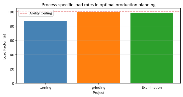
When we can’t secure all orders, we decide on the product lineup based not only on sales but also at marginal profit, delivery times, key customers, and back-end process capabilities. Linear programming clearly identifies “what the bottlenecks are and where the value lies in increasing capacity.”

Approach to Analysis and Modeling

If we $x_j$ the production volume of the product $j$ , $c_j$ unit profit, $a_{ij}$ the required time for process $i$ , and $b_i$ capacity,

\max_{\boldsymbol{x}}\ \boldsymbol{c}^{\mathsf T}\boldsymbol{x} \quad \text{s.t.}\quad A\boldsymbol{x}\leq\boldsymbol{b}, \quad 0\leq x_j\leq d_j

That’s right. Continuous solutions serve as the basis for capacity allocation, but actual lots, setup order, and minimum production quantities are handled using the integer and mixed integer models.

Check with Python

profit = np.array([3200, 5100])
capacity = np.array([780, 850, 520])  # minutes/day
requirements = cycle_minutes.to_numpy()
upper_demand = np.array([70, 50])
plan = linprog(-profit, A_ub=requirements, b_ub=capacity, bounds=list(zip([0, 0], upper_demand)), method="highs")
production_plan = plan.x
used_minutes = requirements @ production_plan

plan_df = pd.DataFrame({
    "Products": products,
    "planned quantity": production_plan,
    "Requirement ceiling": upper_demand,
    "Unit profit (yen)": profit,
})
capacity_df = pd.DataFrame({
    "Project": processes, "Usage time (minutes)": used_minutes,
    "Ability (points)": capacity, "load factor": used_minutes / capacity,
})
display(plan_df.style.format({"planned quantity": "{:.1f}", "Unit profit (yen)": "{:,.0f}"}))
display(capacity_df.style.format({"Usage time (minutes)": "{:.1f}", "load factor": "{:.1%}"}))
print("Daily marginal profit:", f"{profit @ production_plan:,.0f} JPY")

fig, ax = plt.subplots(figsize=(7.4, 4.0))
ax.bar(capacity_df["Project"], capacity_df["load factor"] * 100, color=["steelblue", "tab:orange", "tab:green"])
ax.axhline(100, color="tab:red", linestyle="--", label="Ability Ceiling")
ax.set_title("Process-specific load rates in optimal production planning")
ax.set_xlabel("Project")
ax.set_ylabel("Load Factor (%）")
ax.grid(True, axis="y", alpha=0.3)
ax.legend()
plt.tight_layout()
plt.show()

	Products	planned quantity	Requirement ceiling	Unit profit (yen)
0	Standard productA	46.7	70	3,200
1	High-precision productsB	50.0	50	5,100

	Project	Usage time (minutes)	Ability (points)	load factor
0	turning	680.0	780	87.2%
1	grinding	850.0	850	100.0%
2	Examination	511.7	520	98.4%

Daily Marginal Profit: 404,333 yen

svg

Reading the results

The process where the load rate reaches 100% is the bottleneck in the plan. This serves as a basis for considering adding capacity, shortening cycles, or outsourcing to those processes. However, the linear model averages setup losses, failures, and the order of arrival within the day. Instead of using the optimal value as an on-site instruction, we rounded it into integer lots, reconfirmed the capability constraints, and verified feasibility through the next queue and simulation.

No.074: Queue

Meaning in Practice

Even if there is margin in the inspection process on average, there are waits due to variations in arrival and processing times. Using the queue model, you can estimate the waiting time and number of times when increasing the number of inspectors from one to two.

Approach to Analysis and Modeling

Consider M/M/C with $\lambda$ arrival rate, $\mu$ processing rate per person, and $c$ number of counters. Usage rate is

\rho=\frac{\lambda}{c\mu}<1

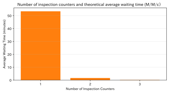
is the stable condition. Using the Erlang C formula, we calculate the waiting probability and average waiting time $W_q$ . Even if the exponential distribution assumption does not fit, it serves as a reference model for understanding the nonlinear relationship between capacity margin and waiting.

Check with Python

def mmc_metrics(arrival_rate, service_rate, servers):
    offered = arrival_rate / service_rate
    rho = offered / servers
    if rho >= 1:
        return {"Number of counters": servers, "utilization rate": rho, "waiting probability": 1.0, "Average Waiting Time_minutes": np.inf, "Mean number within the system": np.inf}
    terms = sum(offered**n / math.factorial(n) for n in range(servers))
    tail = offered**servers / (math.factorial(servers) * (1 - rho))
    p0 = 1 / (terms + tail)
    p_wait = tail * p0
    wq = p_wait / (servers * service_rate - arrival_rate)
    return {"Number of counters": servers, "utilization rate": rho, "waiting probability": p_wait, "Average Waiting Time_minutes": wq * 60, "Mean number within the system": arrival_rate * (wq + 1 / service_rate)}

arrival_rate, service_rate = 8.0, 9.0  # Units/hour
queue_df = pd.DataFrame([mmc_metrics(arrival_rate, service_rate, c) for c in [1, 2, 3]])
display(queue_df.style.format({"utilization rate": "{:.1%}", "waiting probability": "{:.1%}", "Average Waiting Time_minutes": "{:.1f}", "Mean number within the system": "{:.2f}"}))

fig, ax = plt.subplots(figsize=(7.2, 4.0))
ax.bar(queue_df["Number of counters"].astype(str), queue_df["Average Waiting Time_minutes"], color="tab:orange")
ax.set_title("Number of inspection counters and theoretical average waiting time (M/M/c）")
ax.set_xlabel("Number of Inspection Counters")
ax.set_ylabel("Average Waiting Time (minutes)")
ax.grid(True, axis="y", alpha=0.3)
plt.tight_layout()
plt.show()

	Number of counters	utilization rate	waiting probability	Average Waiting Time_minutes	Mean number within the system
0	1	88.9%	88.9%	53.3	8.00
1	2	44.4%	27.4%	1.6	1.11
2	3	29.6%	6.8%	0.2	0.92

svg

Reading the results

Usage rates are high at a single counter, and even slight fluctuations can cause waiting times to spike. Increasing to two reduces average waiting times significantly, but the improvement in the third option is relatively smaller. In practice, we check not only averages but also the 95th percentile, peak hours, inspectors’ concurrent duties, and product-specific inspection times. We compare the costs of staff increase with the amount of delays in delivery and work-in-progress inventory reductions to make judgments.

No.075: Markov Model

Meaning in Practice

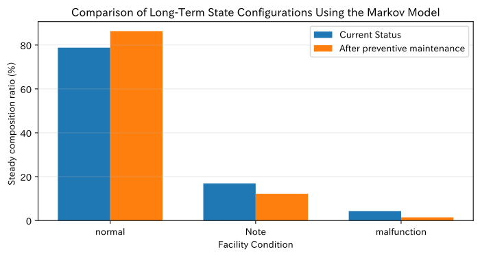
Extending the state transition matrix to long-term operation estimates the proportion of time the equipment is in normal, caution, or failure. If preventive maintenance increases ‘Caution → Normal’ and reduces ‘Caution → Failure,’ you can compare how much long-term utilization rates change.

Approach to Analysis and Modeling

The stationary distribution $\boldsymbol{\pi}$ is

\boldsymbol{\pi}=\boldsymbol{\pi}P, \qquad \sum_i\pi_i=1

It meets the requirements. The left eigenvector corresponding to eigenvalue 1 is used, or calculated through iterative calculations. In finite period investment valuation, transitional changes from the initial state are also important, and decisions are not made solely by steady distribution.

Check with Python

P_preventive = np.array([
    [0.92, 0.075, 0.005],
    [0.48, 0.47, 0.05],
    [0.72, 0.00, 0.28],
])

def stationary_distribution(matrix):
    values, vectors = np.linalg.eig(matrix.T)
    vector = np.real(vectors[:, np.argmin(np.abs(values - 1))])
    return vector / vector.sum()

pi_base = stationary_distribution(P)
pi_pm = stationary_distribution(P_preventive)
markov_compare = pd.DataFrame({"Condition": states, "Current Status": pi_base, "After preventive maintenance": pi_pm})
markov_compare["Difference (pt）"] = (markov_compare["After preventive maintenance"] - markov_compare["Current Status"]) * 100
display(markov_compare.style.format({"Current Status": "{:.1%}", "After preventive maintenance": "{:.1%}", "Difference (pt）": "{:+.1f}"}))

fig, ax = plt.subplots(figsize=(7.4, 4.0))
x = np.arange(len(states))
ax.bar(x - 0.18, pi_base * 100, width=0.36, label="Current Status")
ax.bar(x + 0.18, pi_pm * 100, width=0.36, label="After preventive maintenance")
ax.set_title("Comparison of Long-Term State Configurations Using the Markov Model")
ax.set_xlabel("Facility Condition")
ax.set_ylabel("Steady composition ratio (%）")
ax.set_xticks(x, states)
ax.grid(True, axis="y", alpha=0.3)
ax.legend()
plt.tight_layout()
plt.show()

	Condition	Current Status	After preventive maintenance	Difference (pt）
0	normal	78.8%	86.3%	+7.5
1	Note	16.9%	12.2%	-4.7
2	malfunction	4.3%	1.4%	-2.9

svg

Reading the results

In preventive maintenance scenarios, the proportion of long-term healthy states increases and the proportion of faulty states decreases. Multiplying the difference in failure rates by the number of equipment, daily downtime losses, and annual days creates a rough benefit limit. However, investment profitability is evaluated by including stoppages during maintenance hours, parts costs, initial defects due to maintenance, and confidence intervals for transition probability.

No.076: Discrete Event Simulation

Meaning in Practice

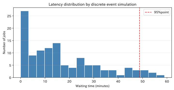
Discrete event simulation processes product arrival, machining start, and machining completion in chronological order. You can reproduce the distribution of wait times that cannot be seen by average values alone, peak congestion during peak periods, and the impact of first-come, first-served rules.

Approach to Analysis and Modeling

Put future events in priority queues and move the clock forward to the earliest event. For a single process, the start and finish times of Job $i$ are

B_i=\max(A_i,C_{i-1}),\qquad C_i=B_i+S_i, \qquad W_i=B_i-A_i

That’s right. Here, we implement this recursion as an event log. With event-driven approaches, breakdowns, repairs, and multiple processes can be added using the same approach.

Check with Python

def single_station_des(n_jobs=120, arrival_mean=7.5, service_mean=6.5, seed=76):
    local_rng = np.random.default_rng(seed)
    arrivals = np.cumsum(local_rng.exponential(arrival_mean, n_jobs))
    services = local_rng.lognormal(np.log(service_mean) - 0.5 * 0.25**2, 0.25, n_jobs)
    available = 0.0
    records = []
    event_queue = []
    for job, (arrival, service) in enumerate(zip(arrivals, services), 1):
        heapq.heappush(event_queue, (arrival, "Arrival", job))
        start = max(arrival, available)
        finish = start + service
        available = finish
        heapq.heappush(event_queue, (finish, "Finished", job))
        records.append([job, arrival, start, finish, start - arrival, service])
    return pd.DataFrame(records, columns=["Jobs", "arrival time", "Start time", "Completion time", "waiting time", "processing time"]), event_queue

des_df, event_queue = single_station_des()
display(des_df.head().style.format({c: "{:.1f}" for c in des_df.columns[1:]}))
display(des_df[["waiting time", "processing time"]].describe(percentiles=[0.5, 0.9, 0.95]).round(2))

fig, ax = plt.subplots(figsize=(7.6, 4.0))
ax.hist(des_df["waiting time"], bins=18, color="steelblue", edgecolor="white")
ax.axvline(des_df["waiting time"].quantile(0.95), color="tab:red", linestyle="--", label="95%point")
ax.set_title("Latency distribution by discrete event simulation")
ax.set_xlabel("Waiting time (minutes)")
ax.set_ylabel("Number of jobs")
ax.grid(True, axis="y", alpha=0.3)
ax.legend()
plt.tight_layout()
plt.show()

	Jobs	arrival time	Start time	Completion time	waiting time	processing time
0	1	13.8	13.8	21.1	0.0	7.3
1	2	28.5	28.5	38.6	0.0	10.1
2	3	34.7	38.6	44.2	3.9	5.6
3	4	43.9	44.2	51.0	0.4	6.8
4	5	44.1	51.0	57.6	6.9	6.6

	waiting time	processing time
count	120.00	120.00
mean	17.25	6.46
std	15.44	1.57
min	0.00	3.52
50%	13.54	6.50
90%	42.94	8.33
95%	48.76	9.81
max	58.99	11.55

svg

Reading the results

You can check not only the average waiting time but also the length of jobs waiting long. For delivery times and buffer design, 90% to 95% points are more useful than average. This example is a single facility that omits breakdowns and breaks. In the production model, the distribution of arrival intervals and machining times is verified from the performance logs, and priority products, arrangements, reprocessing, and shift boundaries are added within the necessary range.

No.077: Monte Carlo Method

Meaning in Practice

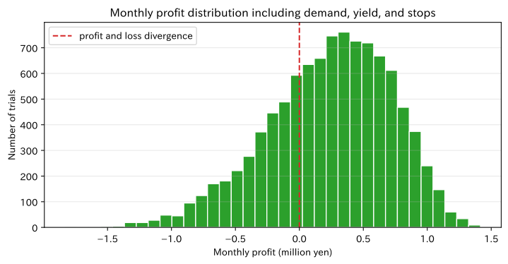
In business plans, demand, yield, and downtime tend to be fixed at a single assumed value. The Monte Carlo method repeatedly samples multiple uncertainties and shows not only the expected profit value but also the probability of losses and downside swings.

Approach to Analysis and Modeling

Calculate KPI $Y=g(\boldsymbol{X})$ from uncertain input $\boldsymbol{X}$ and approximate the distribution with $N$ sample $Y^{(1)},\ldots,Y^{(N)}$ .

\widehat{E[Y]}=\frac{1}{N}\sum_{r=1}^NY^{(r)}, \qquad \widehat{\Pr}(Y<y_0)=\frac{1}{N}\sum_{r=1}^N\mathbf{1}(Y^{(r)}<y_0)

Even if you increase the number of iterations, the error in the input distribution will not be corrected. We define distribution, intervariate correlation, and extreme events based on field data and insights.

Check with Python

n_sim = 10_000
mc_rng = np.random.default_rng(77)
monthly_demand = np.maximum(0, mc_rng.normal(1450, 180, n_sim))
yield_rate = np.clip(mc_rng.beta(90, 6, n_sim), 0, 1)
downtime_hours = mc_rng.gamma(shape=2.2, scale=7.0, size=n_sim)
capacity_units = np.maximum(0, 1600 - downtime_hours * 5.5)
good_units = np.minimum(monthly_demand, capacity_units) * yield_rate
sales = good_units * 8_200
variable_cost = np.minimum(monthly_demand, capacity_units) * 4_600
fixed_cost = 4_100_000
profit_mc = sales - variable_cost - fixed_cost

mc_kpi = pd.DataFrame({
    "KPI": ["average profit", "interest5%point", "interest95%point", "deficit probability"],
    "value": [profit_mc.mean(), np.quantile(profit_mc, 0.05), np.quantile(profit_mc, 0.95), np.mean(profit_mc < 0)],
})
display(mc_kpi.style.format({"value": lambda x: f"{x:,.0f}" if abs(x) > 1 else f"{x:.1%}"}))

fig, ax = plt.subplots(figsize=(7.6, 4.0))
ax.hist(profit_mc / 1e6, bins=35, color="tab:green", edgecolor="white")
ax.axvline(0, color="tab:red", linestyle="--", label="profit and loss divergence")
ax.set_title("Monthly profit distribution including demand, yield, and stops")
ax.set_xlabel("Monthly profit (million yen)")
ax.set_ylabel("Number of trials")
ax.grid(True, axis="y", alpha=0.3)
ax.legend()
plt.tight_layout()
plt.show()

	KPI	value
0	average profit	233,893
1	interest5%point	-657,416
2	interest95%point	948,985
3	deficit probability	29.6%

svg

Reading the results

Even if the average profit is positive, looking at the lower 5% points or the probability of losses shows the safety margin in decision-making. Capital investment proposals are compared not only by increasing average profits but also by how much to reduce the probability of losses and the probability of missing deliveries. In practice, we examine the correlations between demand and price, and between stops and yields, and evaluate long-term out-of-distribution stops separately as stress scenarios.

No.078: Digital Twin

Meaning in Practice

A digital twin is a system that continuously captures the situation on site and tests measures while updating differences from virtual models. It focuses not on 3D display itself, but on synchronization with reality, calibration, discrepancy monitoring, and connection to decision-making.

Approach to Analysis and Modeling

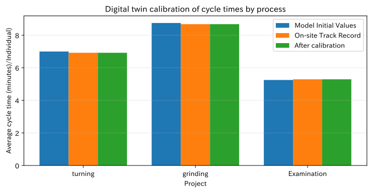
The calibration coefficients for the model average cycle $m_i$ and actual average $\bar{x}_i$ for process $i$

k_i=\frac{\bar{x}_i}{m_i},\qquad m_i^{\mathrm{updated}}=k_im_i

Let’s say so. Even simple ratio calibration can identify which steps of the virtual model are optimistic. Separate calibration data from validation data, and confirm whether different periods can be reproduced after the update.

Check with Python

model_cycle = cycle_minutes.mean(axis=1).to_numpy()
actual_cycle = np.array([observed_cycle[p].mean() for p in processes])
calibration = actual_cycle / model_cycle
updated_cycle = model_cycle * calibration
twin_df = pd.DataFrame({
    "Project": processes,
    "Model Initial Value (minutes)": model_cycle,
    "Actual average (minutes)": actual_cycle,
    "correction factor": calibration,
    "After update (minutes)": updated_cycle,
    "Initial differences (%）": (model_cycle / actual_cycle - 1) * 100,
})
display(twin_df.style.format({c: "{:.2f}" for c in twin_df.columns[1:]}))

fig, ax = plt.subplots(figsize=(7.8, 4.1))
x = np.arange(len(processes))
ax.bar(x - 0.26, model_cycle, width=0.26, label="Model Initial Values")
ax.bar(x, actual_cycle, width=0.26, label="On-site Track Record")
ax.bar(x + 0.26, updated_cycle, width=0.26, label="After calibration")
ax.set_title("Digital twin calibration of cycle times by process")
ax.set_xlabel("Project")
ax.set_ylabel("Average cycle time (minutes)/Individual)")
ax.set_xticks(x, processes)
ax.grid(True, axis="y", alpha=0.3)
ax.legend()
plt.tight_layout()
plt.show()

	Project	Model Initial Value (minutes)	Actual average (minutes)	correction factor	After update (minutes)	Initial differences (%）
0	turning	7.00	6.92	0.99	6.92	1.14
1	grinding	8.75	8.68	0.99	8.68	0.83
2	Examination	5.25	5.29	1.01	5.29	-0.78

svg

Reading the results

In processes where the calibration factor is greater than 1, the early model optimistically represents the on-site situation. The average matches after the update, but this does not mean validation is complete. Errors in variance, time zones, product configuration, and failure frequency are checked over separate periods. Twins can only be operated after managing alignment of equipment IDs, time, and units, sensor shortages, model versions, and update approvers.

No.079: Optimization

Meaning in Practice

Even if there are multiple improvement options, the budget and personnel are limited. We organize the costs and expected reduction losses for each initiative, and select the portfolio that maximizes effectiveness within the budget, including combinations that cannot be implemented simultaneously.

Approach to Analysis and Modeling

Let the binary variable $x_j\in\{0,1\}$ determine whether to adopt Initiative $j$ , and for benefit $v_j$ , cost $c_j$ , and budget $B$ ,

\max \sum_jv_jx_j \quad\text{s.t.}\quad \sum_jc_jx_j\leq B

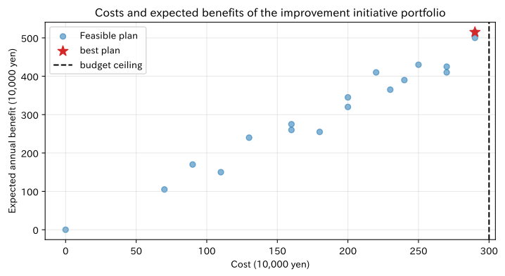
Solve it. Benefits are estimated through simulations and actual results, with constraints on synergies, exclusion conditions, and the number of execution personnel. Since there are few candidates here, we will list all combinations and compare them transparently.

Check with Python

actions = pd.DataFrame({
    "policy": ["Testing Support", "Grinding Prevention Maintenance", "Add safety stock", "Shortening the setup process", "Sensor Expansion"],
    "Fees_ten thousand yen": [90, 130, 70, 160, 110],
    "Expected annual benefits_ten thousand yen": [170, 240, 105, 260, 150],
})
budget = 300
portfolios = []
for mask in range(1 << len(actions)):
    selected = [i for i in range(len(actions)) if mask & (1 << i)]
    cost = actions.loc[selected, "Fees_ten thousand yen"].sum()
    benefit = actions.loc[selected, "Expected annual benefits_ten thousand yen"].sum()
    feasible = cost <= budget
    portfolios.append({"policy": "・".join(actions.loc[selected, "policy"]) or "No implementation", "Fees_ten thousand yen": cost, "benefit_ten thousand yen": benefit, "Within budget": feasible})
portfolio_df = pd.DataFrame(portfolios)
best_portfolio = portfolio_df[portfolio_df["Within budget"]].sort_values(["benefit_ten thousand yen", "Fees_ten thousand yen"], ascending=[False, True]).iloc[0]
display(actions)
display(best_portfolio.to_frame("Optimal Portfolio"))

feasible_df = portfolio_df[portfolio_df["Within budget"]]
fig, ax = plt.subplots(figsize=(7.6, 4.2))
ax.scatter(feasible_df["Fees_ten thousand yen"], feasible_df["benefit_ten thousand yen"], alpha=0.55, label="Feasible plan")
ax.scatter(best_portfolio["Fees_ten thousand yen"], best_portfolio["benefit_ten thousand yen"], s=130, marker="*", color="tab:red", label="best plan")
ax.axvline(budget, color="black", linestyle="--", label="budget ceiling")
ax.set_title("Costs and expected benefits of the improvement initiative portfolio")
ax.set_xlabel("Cost (10,000 yen)")
ax.set_ylabel("Expected annual benefit (10,000 yen)")
ax.grid(True, alpha=0.3)
ax.legend()
plt.tight_layout()
plt.show()

	policy	Fees_ten thousand yen	Expected annual benefits_ten thousand yen
0	Testing Support	90	170
1	Grinding Prevention Maintenance	130	240
2	Add safety stock	70	105
3	Shortening the setup process	160	260
4	Sensor Expansion	110	150

	Optimal Portfolio
policy	Inspection support, grinding preventive maintenance, and additional safety stock
Fees_ten thousand yen	290
benefit_ten thousand yen	515
Within budget	True

svg

Reading the results

You can choose combinations within your budget that maximize expected benefits. However, the benefits shown in the table are point estimates. Using the Monte Carlo method, we evaluate the downside and add constraints such as overlapping effects between measures, lead time for implementation, on-site personnel, and downtime. Optimization does not automate management decisions; rather, it is a tool that clarifies assumptions and trade-offs to help build consensus.

No.080: Factory Simulation

Meaning in Practice

Evaluate local improvements across the entire factory. Even if grinding is done quickly, shipments will not increase if inspections become clogged. We integrate the products flowing through three processes, as well as variations and stoppages between each process, and compare the current situation with improvement proposals under the same demand and random number conditions.

Approach to Analysis and Modeling

Job $j$ and process $i$ completion times

C_{ij}=\max(C_{i-1,j},C_{i,j-1})+S_{ij}+D_{ij}

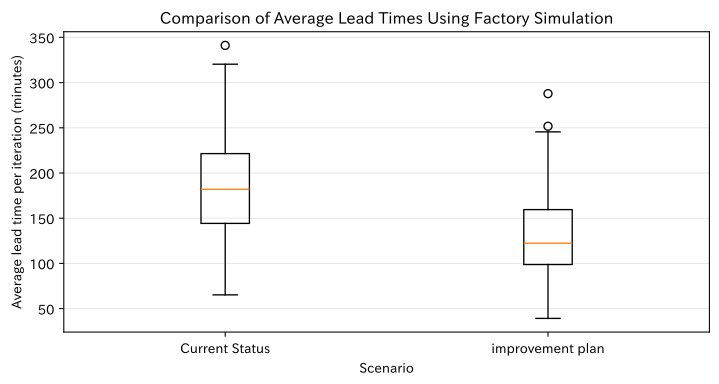
Let’s say so. $S_{ij}$ refers to processing time, and $D_{ij}$ indicates stopping due to malfunction or other reasons. Throughput, lead time, process waiting, and delivery success rate are compared multiple iterations. Using common random numbers suppresses random fluctuations other than policy differences.

Check with Python

def factory_simulation(n_jobs=90, scenario="Current Status", seed=80):
    local_rng = np.random.default_rng(seed)
    arrivals = np.cumsum(local_rng.exponential(7.0, n_jobs))
    base = np.array([7.0, 8.8, 5.2])
    sigma = np.array([0.18, 0.24, 0.20])
    failure_prob = np.array([0.015, 0.040, 0.018])
    repair_mean = np.array([22, 38, 18])
    if scenario == "improvement plan":
        base = base * np.array([1.0, 0.92, 0.88])
        failure_prob = failure_prob * np.array([1.0, 0.45, 1.0])
    available = np.zeros(3)
    records = []
    for job in range(n_jobs):
        previous_finish = arrivals[job]
        waits = []
        for i in range(3):
            start = max(previous_finish, available[i])
            waits.append(start - previous_finish)
            service = local_rng.lognormal(np.log(base[i]) - 0.5 * sigma[i]**2, sigma[i])
            downtime = local_rng.exponential(repair_mean[i]) if local_rng.random() < failure_prob[i] else 0.0
            finish = start + service + downtime
            available[i] = finish
            previous_finish = finish
        lead_time = previous_finish - arrivals[job]
        records.append([job + 1, arrivals[job], previous_finish, lead_time, *waits])
    result = pd.DataFrame(records, columns=["Jobs", "invest", "Finished", "lead time", "waiting for turning", "Waiting for grinding", "Waiting for inspection"])
    horizon = result["Finished"].max() - result["invest"].min()
    kpi = {
        "Throughput (units)/Time)": n_jobs / horizon * 60,
        "Average lead time (minutes)": result["lead time"].mean(),
        "95%Lead time (minutes)": result["lead time"].quantile(0.95),
        "Delivery date60rate within a fraction": np.mean(result["lead time"] <= 60),
    }
    return result, kpi

scenario_rows = []
lead_samples = {"Current Status": [], "improvement plan": []}
for scenario in lead_samples:
    for rep in range(120):
        result, kpi = factory_simulation(scenario=scenario, seed=8000 + rep)
        scenario_rows.append({"Scenario": scenario, "Repeatedly": rep, **kpi})
        lead_samples[scenario].append(kpi["Average lead time (minutes)"])
scenario_df = pd.DataFrame(scenario_rows)
factory_summary = scenario_df.groupby("Scenario").agg({
    "Throughput (units)/Time)": "mean",
    "Average lead time (minutes)": "mean",
    "95%Lead time (minutes)": "mean",
    "Delivery date60rate within a fraction": "mean",
})
display(factory_summary.style.format({
    "Throughput (units)/Time)": "{:.2f}", "Average lead time (minutes)": "{:.1f}",
    "95%Lead time (minutes)": "{:.1f}", "Delivery date60rate within a fraction": "{:.1%}",
}))

fig, ax = plt.subplots(figsize=(7.6, 4.1))
ax.boxplot([lead_samples["Current Status"], lead_samples["improvement plan"]], tick_labels=["Current Status", "improvement plan"])
ax.set_title("Comparison of Average Lead Times Using Factory Simulation")
ax.set_xlabel("Scenario")
ax.set_ylabel("Average lead time per iteration (minutes)")
ax.grid(True, axis="y", alpha=0.3)
plt.tight_layout()
plt.show()

	Throughput (units)/Time)	Average lead time (minutes)	95%Lead time (minutes)	Delivery date60rate within a fraction
Scenario
improvement plan	6.54	129.1	222.6	22.4%
Current Status	5.72	188.4	336.1	15.7%

svg

Reading the results

The improvement plan simultaneously enhances grinding failure probability, machining time, and inspection time, allowing comparison of throughput, average 95% lead time, and on-time delivery rate. The overlapping of the box beard diagram also indicates uncertainty in its effectiveness. Instead of using only average differences, we conduct sensitivity analyses based on improvement costs, confidence intervals for effectiveness, busy periods, long-term shutdowns, and product mix variations. If local KPIs improve but overall KPIs remain unchanged, look for alternative constraint processes.

Practical Implications Seen Through Target Exercise

Defining the state allows for future discussion.: State transition matrices and Markov models allow evaluation of short-term and long-term configurations of equipment groups.
Abilities and fluctuations are treated separately.: Production planning allocates average capacity, while queue and discrete event simulation handle variations in arrival and processing.
Inventory is a condition for service level: Design safety stock based on demand, lead time, and out-of-stock costs, rather than fixed values.
Don’t make investment decisions based solely on averages: Use the Monte Carlo method to check for downside factors such as loss probability, quantiles, and missed delivery dates.
Digital twins are a continuous calibration process.: Measure differences from on-site performance and manage model versions and input quality.
Going back and forth between optimization and simulation: Narrow down candidates through optimization and verify dynamic feasibility through simulation.
OverallKPIEvaluating Local Improvements: We track not only process uptime but also shipment volume, lead time, work-in-progress, and profit.

What is necessary for practical implementation

1. Define judgments and KPIs in advance

Decisions such as “whether to increase the number of inspectors,” “how many safety stock to maintain,” and “which equipment to maintain for maintenance” are clarified. Calculate throughput, on-time completion rate, work-in-progress inventory, shortage costs, and stoppage losses within the scope and units.

2. Organize the time, status, and events of the data

The equipment ID, part number, lot, process, machining start/finish, stop reason, and repair completion are connected by a common key. It distinguishes between missing measurements and zeros, planned stoppages and fault stops, reprocessing and new processing, and records the history of equipment and process changes.

3. Validate the model step by step

Based on manual calculations and queues, proceed to discrete events only when necessary. By comparing average and variance by process, daily shipments, WIP, and number of stops against actual performance, reproducibility is confirmed even during periods not used for calibration, busy periods, or abnormal periods.

4. Show uncertainty and sensitivity

Consider the distribution and correlation of demand, processing time, breakdown, and repair time. Instead of a single result, quantiles, confidence intervals, and stress scenarios are presented, and sensitivity analysis is used to identify inputs that influence conclusions.

5. Design decision-making and update operations

Decide on the approver of the model, the frequency of input updates, the conditions for recalibration, and the person responsible for implementing improvement proposals. Post-implementation KPIs are recorded, and the difference between predicted and actual benefits is returned to the next model. Simulation is managed as a common language between the field and management.

Conclusion

From No.071 to No.080, we examined hypothetical precision component lines to examine state transition matrices, inventory models, production planning, queues, Markov models, discrete event simulations, Monte Carlo method, digital twins, optimization of improvement measures, and whole-factory simulation.

The key to leveraging simulation in manufacturing is not simply creating sophisticated models. Defining decision-making, verifying models based on field performance, showing uncertainty, and then returning the results after measures to the next judgment..

Consultations for Corporations

At Mathematical Laboratory, we support everything from problem organization to data design, PoC, validation verification, and on-site operations in manufacturing industry state transition analysis, inventory and production planning, queue analysis, discrete event simulation, Monte Carlo evaluation, digital twin, and mathematical optimization.

You can consult us about issues such as “wanting to identify bottlenecks before expanding equipment,” “quantifying the balance between inventory and out-of-stock,” “linking factory simulations to investment decisions,” or “improving the gap between existing simulations and on-site performance.”

📩 Contact Us: surikobo.co.jp/contact
Please feel free to consult us first.

Factory Simulation Implemented with Python | Decision-Making for Inventory, Queues, and Production Planning

Designing processing lines resistant to fluctuations

State transition, inventory, queues, factory simulation: 100 Exercises No.071–No.080

Introduction: Practical Challenges in Manufacturing Covered in This Article

Common situations on site

Why is this issue so difficult to judge?

Overview of Exercise covered this time

Preparing the Python environment

Creation of Fictional Data

No.071: State Transition Matrix

Meaning in Practice

Approach to Analysis and Modeling

Check with Python

Reading the results

No.072: Stock Model

Meaning in Practice

Approach to Analysis and Modeling

Check with Python

Reading the results

No.073: Production Plan

Meaning in Practice

Approach to Analysis and Modeling

Check with Python

Reading the results

No.074: Queue

Meaning in Practice

Approach to Analysis and Modeling

Check with Python

Reading the results

No.075: Markov Model

Meaning in Practice

Approach to Analysis and Modeling

Check with Python

Reading the results

No.076: Discrete Event Simulation

Meaning in Practice

Approach to Analysis and Modeling

Check with Python

Reading the results

No.077: Monte Carlo Method

Meaning in Practice

Approach to Analysis and Modeling

Check with Python

Reading the results

No.078: Digital Twin

Meaning in Practice

Approach to Analysis and Modeling

Check with Python

Reading the results

No.079: Optimization

Meaning in Practice

Approach to Analysis and Modeling

Check with Python

Reading the results

No.080: Factory Simulation

Meaning in Practice

Approach to Analysis and Modeling

Check with Python

Reading the results

Practical Implications Seen Through Target Exercise

What is necessary for practical implementation

1. Define judgments and KPIs in advance

2. Organize the time, status, and events of the data

3. Validate the model step by step

4. Show uncertainty and sensitivity

5. Design decision-making and update operations

Conclusion

Consultations for Corporations

Related Posts

Introduction to Python Acceleration in Manufacturing | CuPy, JAX, Polars, and Practical Matrix Computation

Integrating Quality, Demand, and Production Planning in Manufacturing with Python | Learning Matrix Analysis in Practice

Learning predictive maintenance in manufacturing with Python | Practical applications of Transformer, GNN, and matrix decomposition

Learning Manufacturing Quality Forecasting with Python | Introduction to Ridge, Logistic Regression, and Attention

Introduction to Process Network Analysis in Manufacturing | Learning PCA, PageRank, and GCN with Python