An Introduction to Probability Distinguishing Between ‘Chance’ and ‘Structure’ in Defect Rates: 10 Exercises to Learn with Manufacturing Quality Data

This article is a practical notebook that teaches the foundation of probability theory, Events, probability axioms, conditional probability, independence, Bayes’ theorem, law of large numbers, through continuous decision-making, focusing on quality control in manufacturing. Using fictitious inspection records obtained from three production lines, we use Python to check “what the overall defect rate hides,” “which line should be prioritized when defective products are found,” and “how much to trust in preliminary values with small sample sizes.”

This “100 Exercises on Probability and Statistical Theory” series is not about memorizing formulas, but about mathematically explaining decisions about manufacturing, quality, maintenance, and supply and demand. The first 10 questions establish a common language to support subsequent probability distributions, estimations, and tests.

[!NOTE] This material is a notebook previously used by Surikoubo (or personally by the representative, Kazuyama), and has been reconstructed, edited, and published with the company’s permission.
All data listed is fictional and has no relation whatsoever to real companies, factories, or figures.

Introduction: Practical Challenges in Manufacturing Covered in This Article

At the quality meeting, the overall value is first reported: “This month’s defect rate was 3.1%.” However, the necessary decisions lie beyond that. You must distinguish whether defects increased during night shifts, changes in the composition ratio of specific lines, where to start investigating the causes of defective products, and whether the observed differences are merely coincidence with a small amount of data.

The goal of this article is to be able to treat probability not just as a percentage, but as a Decision Measures Specifying Scope (Sample Space) and Conditions.

Common situations on site

• Even though production numbers differ by line and shift, priorities are determined solely by the number of simple defects.
• They do not look at the overlap between “night shifts” and “delinquents,” but only compare the respective proportions
• Since many defective products originate from Line A, they judge that the quality of Line A is the worst.
• The defect rate for the day is determined by the results of dozens of tests in the morning.
• The denominator, exclusion criteria, and handling of missing data on dashboards vary by department.

These can be organized using basic concepts such as sets, conditional probability, total probability, and Bayesian updates.

Why is this issue so difficult to judge?

First, the defect rate is the ratio of “number of defective products to number of inspections,” and the value changes when the product set, which serves as the denominator, changes. Second, the composition ratio of lines and shifts, as well as the defect rates under each condition, simultaneously affect the overall value. Third, with a finite number of tests, sample variation is unavoidable.

Therefore, before analysis, it is necessary to define $Omega$ (all products to be targeted), event $A$ (set of products of interest), and condition $B$ (comparison target), and finally check for uncertainty based on sample size.

Overview of Exercise covered this time

No.	Theme	Questions in the Manufacturing Industry
001	Sets and Events	How to define defects, night shifts, and lines
002	specimen space	Which product group should be used as the denominator in probability calculations?
003	axiom of probability	What alignment should probability as a KPI satisfy
004	addition theorem	How to eliminate duplicates of “bad or night shift”
005	Conditional probability	Here are some defect rates limited to night shifts:
006	Multiplication theorem	Can the conditions be decomposed sequentially to obtain simultaneous occurrence?
007	independent event	Is it acceptable to consider night shifts and defective work as unrelated?
008	Total probability theorem	Can the overall defect rate be reconstructed from the line-by-line defect rate?
009	Bayes’ theorem	How does the manufacturing line’s potential change after observing defective products?
010	Monte Carlo Method and the Law of Large Numbers	How do preliminary data values stabilize when the number of tests increases?

Preparing the Python environment

It does not rely on external data, using only numpy, pandas, and matplotlib. Because it fixes the random number seed, even if you rerun, you will get the same fictional data and diagram.

import sys
import numpy as np
import pandas as pd
import matplotlib
import matplotlib.pyplot as plt
import japanize_matplotlib
from IPython.display import display

SEED = 20260711
rng = np.random.default_rng(SEED)
plt.rcParams["figure.figsize"] = (8, 4.5)
plt.rcParams["axes.unicode_minus"] = False

print(f"Python     : {sys.version.split()[0]}")
print(f"NumPy      : {np.__version__}")
print(f"pandas     : {pd.__version__}")
print(f"Matplotlib : {matplotlib.__version__}")
print(f"random seed: {SEED}")

Python     : 3.13.1
NumPy      : 2.5.1
pandas     : 3.0.3
Matplotlib : 3.11.0
random seed: 20260711

Creation of Fictional Data

For 12,000 products, it generates production line data, shifts, equipment temperature ranges, and defect status. The base defect probability varies by line, and the defect probability increases during night shifts and high temperatures. This is not data proving causality, but rather a hypothetical scenario to confirm the concept of probability.

n_units = 12_000
line = rng.choice(["A", "B", "C"], size=n_units, p=[0.45, 0.35, 0.20])
shift = rng.choice(["day shift", "night shift"], size=n_units, p=[0.70, 0.30])
temperature = rng.choice(["usually", "high temperature"], size=n_units, p=[0.88, 0.12])

base_rate = pd.Series(line).map({"A": 0.015, "B": 0.030, "C": 0.050}).to_numpy()
defect_probability = base_rate + (shift == "night shift") * 0.012 + (temperature == "high temperature") * 0.018
is_defect = rng.random(n_units) < defect_probability

df = pd.DataFrame({
    "product_id": [f"P{i:05d}" for i in range(1, n_units + 1)],
    "line": line,
    "shift": shift,
    "temperature": temperature,
    "is_defect": is_defect,
})
df["result"] = np.where(df["is_defect"], "bad", "good product")

display(df.head())
summary = (df.groupby(["line", "shift"], observed=True)
             .agg(number_of_inspections=("product_id", "size"), number_of_defects=("is_defect", "sum"), non_performing_rate=("is_defect", "mean")))
display(summary.style.format({"non_performing_rate": "{:.2%}"}))

	product_id	line	shift	temperature	is_defect	result
0	P00001	A	day shift	high temperature	False	good product
1	P00002	C	day shift	usually	False	good product
2	P00003	B	day shift	usually	False	good product
3	P00004	B	day shift	high temperature	False	good product
4	P00005	C	day shift	usually	False	good product

		number_of_inspections	number_of_defects	non_performing_rate
line	shift
A	night shift	1618	36	2.22%
	day shift	3786	58	1.53%
B	night shift	1281	52	4.06%
	day shift	2955	108	3.65%
C	night shift	673	45	6.69%
	day shift	1687	73	4.33%

From the generated results, it is clear that the number of inspections and defect rates vary depending on the line and shift. From then on, the same data is interpreted with different probability concepts to check which decisions each concept supports.

No.001: Sets and Events

Meaning in Practice

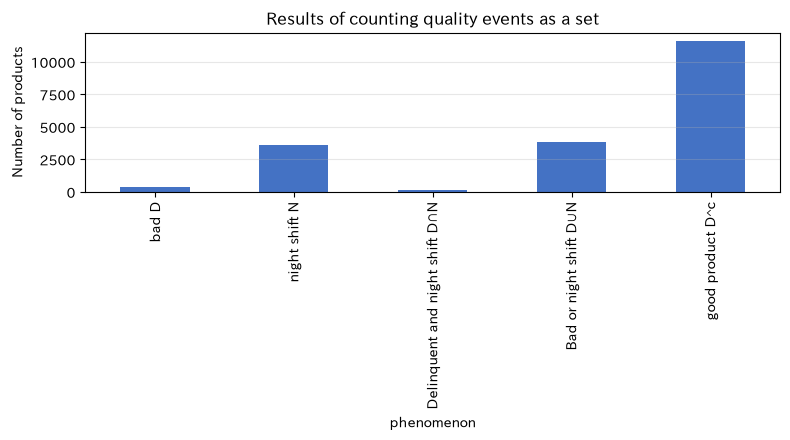
By defining quality conditions as a set, you can clearly express complex conditions such as “defective and night shift” or “defective or high temperature.” We also support the specifications for data extraction conditions as is.

Approach to Analysis and Modeling

All inspection products are $Omega$, defective product events are $D$, and night shift products are $N$. Common parts $D\cap N$ are defective items for night shifts, union $D\cup N$ are defective or night shift products, and complementary $D^c$ are good products. An event is not a result of “whether it happens or doesn’t happen,” but rather a collection of samples that meet certain conditions.

Check with Python

D = set(df.loc[df["is_defect"], "product_id"])
N = set(df.loc[df["shift"] == "night shift", "product_id"])
omega = set(df["product_id"])

set_counts = pd.Series({
    "bad D": len(D),
    "night shift N": len(N),
    "Delinquent and night shift D∩N": len(D & N),
    "Bad or night shift D∪N": len(D | N),
    "good product D^c": len(omega - D),
})
display(set_counts.to_frame("Number of products"))

set_counts.plot(kind="bar", color="#4472C4")
plt.title("Results of counting quality events as a set")
plt.xlabel("phenomenon")
plt.ylabel("Number of products")
plt.grid(axis="y", alpha=0.3)
plt.tight_layout()
plt.show()

	Number of products
bad D	372
night shift N	3572
Delinquent and night shift D∩N	133
Bad or night shift D∪N	3811
good product D^c	11628

Reading the results

Since “defective” and “night shift” overlap, the sum of the number of cases for both does not count as the number of “defective or night shift” cases. The KPI extraction conditions require defining AND, OR, NOT, and the denominator simultaneously.

No.002: What is a Specimen Space?

Meaning in Practice

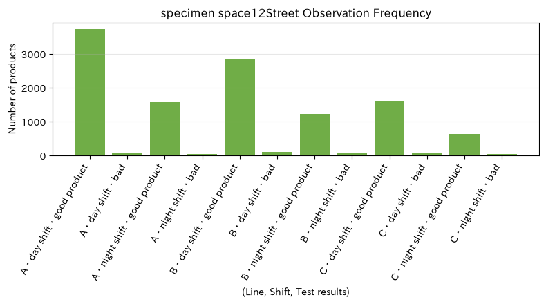
A sample space is a collection that collects all possible outcomes from probabilistic calculations. If the target month, target factory, or whether re-inspection items are included, the sample space will also change, and the meaning of the defect rate for comparison will also change.

Approach to Analysis and Modeling

Here, the results for one product are represented in $(\text{line},\text{shift},\text{result})$. With three lines, two shifts, and two test results, the theoretical sample space is $3\times2\times2=12$. Each product belongs to one of the following elements.

Check with Python

from itertools import product

sample_space = list(product(["A", "B", "C"], ["day shift", "night shift"], ["good product", "bad"]))
observed = (df.groupby(["line", "shift", "result"], observed=False)
              .size().reindex(pd.MultiIndex.from_tuples(sample_space), fill_value=0))
space_table = observed.rename("Number of products").reset_index()
space_table.columns = ["Line", "Shift", "Results", "Number of products"]
display(space_table)

labels = space_table["Line"] + "・" + space_table["Shift"] + "・" + space_table["Results"]
plt.bar(labels, space_table["Number of products"], color="#70AD47")
plt.title("specimen space12Street Observation Frequency")
plt.xlabel("(Line, Shift, Test results)")
plt.ylabel("Number of products")
plt.xticks(rotation=60, ha="right")
plt.grid(axis="y", alpha=0.3)
plt.tight_layout()
plt.show()

	Line	Shift	Results	Number of products
0	A	day shift	good product	3728
1	A	day shift	bad	58
2	A	night shift	good product	1582
3	A	night shift	bad	36
4	B	day shift	good product	2847
5	B	day shift	bad	108
6	B	night shift	good product	1229
7	B	night shift	bad	52
8	C	day shift	good product	1614
9	C	day shift	bad	73
10	C	night shift	good product	628
11	C	night shift	bad	45

Reading the results

By specifying 12 ways, you can monitor combinations that do not exist in the data. In practice, it is important to distinguish whether a “zero observation count” could not have occurred, happened to be absent this month, or was not collected.

No.003: Probability Axioms

Meaning in Practice

Before combining multiple quality KPIs, check whether they are consistent as probabilities. If the proportion is negative, the total of all categories is not 100%, or the total of non-duplicated categories does not match the total, there may be issues with aggregation specifications or data quality.

Approach to Analysis and Modeling

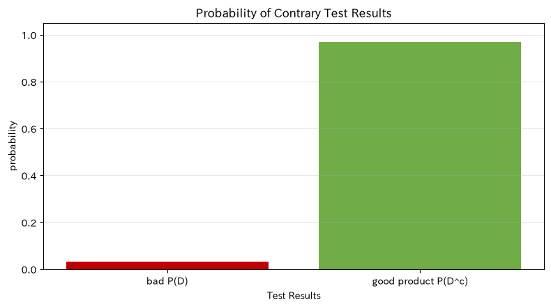
Probability $P$ satisfies $P(\cup_i A_i)=\sum_i P(A_i)$ for (1) $P(A)\geq0$, (2) $P(\Omega)=1$, and (3) mutually exclusive $A_i$. Good $D^c$ and bad $D$ are exclusions, and their union is $Omega$.

Check with Python

p_defect = df["is_defect"].mean()
p_pass = 1 - p_defect
p_omega = len(omega) / len(omega)

axioms = pd.DataFrame({
    "Confirmation items": ["non-negative P(D) ≥ 0", "whole event P(Ω) = 1", "exclusion addition P(D)+P(D^c)=P(Ω)"],
    "left side": [p_defect, p_omega, p_defect + p_pass],
    "expected value": [0.0, 1.0, 1.0],
    "determination": [p_defect >= 0, np.isclose(p_omega, 1), np.isclose(p_defect + p_pass, 1)],
})
display(axioms.style.format({"left side": "{:.4f}", "expected value": "{:.4f}"}))

plt.bar(["bad P(D)", "good product P(D^c)"], [p_defect, p_pass], color=["#C00000", "#70AD47"])
plt.title("Probability of Contrary Test Results")
plt.xlabel("Test Results")
plt.ylabel("probability")
plt.ylim(0, 1.05)
plt.grid(axis="y", alpha=0.3)
plt.tight_layout()
plt.show()

	Confirmation items	left side	expected value	determination
0	non-negative P(D) ≥ 0	0.0310	0.0000	True
1	whole event P(Ω) = 1	1.0000	1.0000	True
2	exclusion addition P(D)+P(D^c)=P(Ω)	1.0000	1.0000	True

Reading the results

The probabilities of good and defective products are non-negative, with a total of 1. Although the axiom seems obvious, it can be used as a checkout rule to detect duplicates or missing classifications, such as ETL processing and automated testing of quality dashboards.

No.004: Derivation of the Addition Formula

Meaning in Practice

This formula is used to avoid double-counting duplicate items when concluding target conditions with OR conditions, such as “Focus on defective or night shift products.” This directly leads to estimates of required labor and isolation space.

Approach to Analysis and Modeling

The addition formula for two events is as follows.

$P(D\cup N)=P(D)+P(N)-P(D\cap N)$

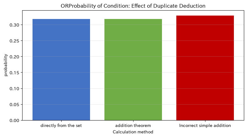
If you simply add $D$ and $N$, you count the common parts twice, so subtract the one time. If it’s rebellion, the common part is zero, and you can calculate it using just the sum of probabilities.

Check with Python

p_D = len(D) / n_units
p_N = len(N) / n_units
p_D_and_N = len(D & N) / n_units
p_union_direct = len(D | N) / n_units
p_union_formula = p_D + p_N - p_D_and_N

addition = pd.DataFrame({
    "calculate": ["directly from the set", "addition theorem", "Incorrect simple addition"],
    "probability": [p_union_direct, p_union_formula, p_D + p_N],
})
display(addition.style.format({"probability": "{:.2%}"}))

plt.bar(addition["calculate"], addition["probability"], color=["#4472C4", "#70AD47", "#C00000"])
plt.title("ORProbability of Condition: Effect of Duplicate Deduction")
plt.xlabel("Calculation method")
plt.ylabel("probability")
plt.grid(axis="y", alpha=0.3)
plt.tight_layout()
plt.show()

	calculate	probability
0	directly from the set	31.76%
1	addition theorem	31.76%
2	Incorrect simple addition	32.87%

Reading the results

Direct aggregation and addition theorems coincide, but only simple addition is excessive by the share of the common part. When estimating the number of isolations or re-inspection man-hours for target products, overlaps between conditions are always deducted.

No.005: Conditional Probability

Meaning in Practice

Instead of the overall defect rate, if you calculate the defect rate under the condition that the product was manufactured during night shifts, you can compare shift-specific risks. Setting conditions means narrowing down the denominator to the night shift product.

Approach to Analysis and Modeling

$P(N)>0$, the conditional probability is

$P(D\mid N)=\frac{P(D\cap N)}{P(N)}$

That’s right. The numerator is night shift and defective, and the denominator is all night shift products. $P(D\mid N)$ and $P(N\mid D)$ have different denominators, so they should not be confused.

Check with Python

conditional_rates = (df.groupby("shift", observed=True)["is_defect"]
                       .agg([("number_of_inspections", "size"), ("number_of_defects", "sum"), ("Conditional defect rate", "mean")]))
display(conditional_rates.style.format({"Conditional defect rate": "{:.2%}"}))

p_D_given_N_formula = p_D_and_N / p_N
print(f"According to the definition formula P(bad | night shift) = {p_D_given_N_formula:.2%}")

conditional_rates["Conditional defect rate"].plot(kind="bar", color=["#5B9BD5", "#ED7D31"])
plt.title("Defect rate conditioned by shift")
plt.xlabel("Shift")
plt.ylabel("non_performing_rate")
plt.xticks(rotation=0)
plt.grid(axis="y", alpha=0.3)
plt.tight_layout()
plt.show()

	number_of_inspections	number_of_defects	Conditional defect rate
shift
night shift	3572	133	3.72%
day shift	8428	239	2.84%

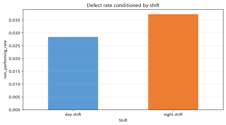
P (Defective | Night Shift) by Definition = 3.72%

Reading the results

The conditional defect rate for night shifts is higher than for day shifts. However, while this serves as the basis for priority investigation, it does not prove that night shifts are the cause of the defect. Additional confounding factors such as line configuration, temperature, and working conditions are checked.

No.006: Multiplication Theorem

Meaning in Practice

The percentage of “night shift products and defects” is estimated by dividing the process step by step. Used to estimate the number of defective products and losses from the night shift ratio and defect rate in the production plan.

Approach to Analysis and Modeling

Redefining conditional probability, the multiplication theorem

$P(N\cap D)=P(N)P(D\mid N)$

You will get it. Generally, the same simultaneous probability is achieved for rearranged $P(D)P(N\mid D)$.

Check with Python

p_N_given_D = p_D_and_N / p_D
multiplication = pd.DataFrame({
    "How to Find": ["direct aggregation", "P(night shift)×P(bad|night shift)", "P(bad)×P(night shift|bad)"],
    "simultaneous probability": [p_D_and_N, p_N * p_D_given_N_formula, p_D * p_N_given_D],
})
display(multiplication.style.format({"simultaneous probability": "{:.4%}"}))

plt.bar(multiplication["How to Find"], multiplication["simultaneous probability"], color=["#4472C4", "#70AD47", "#A5A5A5"])
plt.title("Probability of night shift and defect according to multiplication theorem")
plt.xlabel("Calculation Path")
plt.ylabel("simultaneous probability")
plt.xticks(rotation=12)
plt.grid(axis="y", alpha=0.3)
plt.tight_layout()
plt.show()

	How to Find	simultaneous probability
0	direct aggregation	1.1083%
1	P(night shift)×P(bad|night shift)	1.1083%
2	P(bad)×P(night shift|bad)	1.1083%

Reading the results

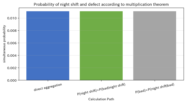
All three paths have the same value. In practice, even at the planning stage when direct simultaneous cases are not yet available, if there is a production composition ratio and conditional defect rate, the expected occurrence can be broken down and explained.

No.007: Independent Events

Meaning in Practice

If two events can be assumed to be independent, the model becomes simpler, but incorrect independent assumptions underestimate the potential for defects. Determining whether shifts and defects are independent relates to the prioritization of staffing and equipment condition surveys.

Approach to Analysis and Modeling

If $D$ and $N$ are independent,

$P(D\cap N)=P(D)P(N)$

and $P(D\mid N)=P(D)$ holds. Since finite data do not provide perfect matching, here we will check the difference and ratio as diagnostic quantities. Formal judgments require confidence intervals and hypothesis testing, which are discussed in subsequent chapters.

Check with Python

independence = pd.DataFrame({
    "indicator": ["Observation P(D∩N)", "Independent assumption P(D)P(N)", "Overall P(D)", "night shift P(D|N)"],
    "probability": [p_D_and_N, p_D * p_N, p_D, p_D_given_N_formula],
})
display(independence.style.format({"probability": "{:.3%}"}))
print(f"Relative Risks of Night Shifts P(D|N) / P(D) = {p_D_given_N_formula / p_D:.2f} double")

plt.bar(independence["indicator"], independence["probability"], color=["#ED7D31", "#A5A5A5", "#4472C4", "#C00000"])
plt.title("Comparison of Independent Assumptions and Observation Probabilities")
plt.xlabel("Probability indicator")
plt.ylabel("probability")
plt.xticks(rotation=18)
plt.grid(axis="y", alpha=0.3)
plt.tight_layout()
plt.show()

	indicator	probability
0	Observation P(D∩N)	1.108%
1	Independent assumption P(D)P(N)	0.923%
2	Overall P(D)	3.100%
3	night shift P(D|N)	3.723%

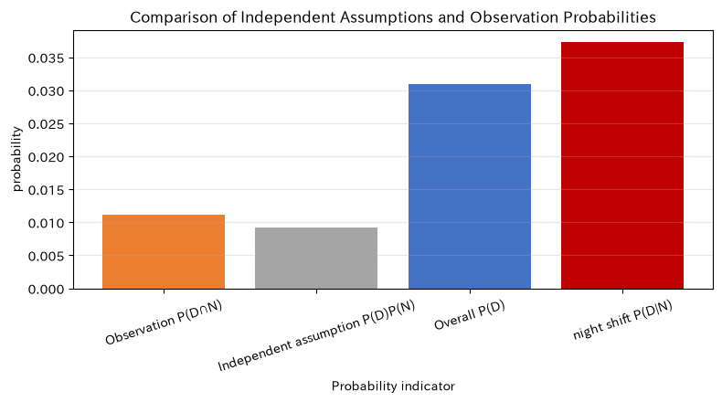
Relative risk of night shifts P(D|N) / P(D) = 1.20 times

Reading the results

The night shift defect rate does not match the overall defect rate, and the observed concurrent probability is larger than the product of independent assumptions. With this data, it is safe to manage it at least by shift, without assuming independence. However, further analysis is needed to identify the causes of the difference.

No.008: Total Probability Theorem

Meaning in Practice

The overall defect rate is not a simple average of defect rates per line. This is an average weighted by the production composition ratio of each line. Therefore, even if equipment improvements do not change defect rates on each line, the overall defect rate changes simply by transferring production.

Approach to Analysis and Modeling

When line $L_i$ divides the sample space without duplication,

$P(D)=\sum_i P(D\mid L_i)P(L_i)$

That’s right. Each item represents the “simultaneous probability of defective products coming from that line,” and also contributes to the overall defect rate.

Check with Python

line_stats = (df.groupby("line", observed=True)["is_defect"]
                .agg([("number_of_inspections", "size"), ("number_of_defects", "sum"), ("Line Defect Rate", "mean")]))
line_stats["Production Composition Ratio"] = line_stats["number_of_inspections"] / n_units
line_stats["Contribution to the overall defect rate"] = line_stats["Production Composition Ratio"] * line_stats["Line Defect Rate"]
display(line_stats.style.format({
    "Line Defect Rate": "{:.2%}", "Production Composition Ratio": "{:.2%}", "Contribution to the overall defect rate": "{:.2%}"
}))
print(f"Total contribution = {line_stats['Contribution to the overall defect rate'].sum():.2%}")
print(f"direct aggregation P(D) = {p_D:.2%}")

line_stats["Contribution to the overall defect rate"].plot(kind="bar", color="#5B9BD5")
plt.title("Contribution to overall defect rates by line")
plt.xlabel("Line")
plt.ylabel("contribution degree")
plt.xticks(rotation=0)
plt.grid(axis="y", alpha=0.3)
plt.tight_layout()
plt.show()

	number_of_inspections	number_of_defects	Line Defect Rate	Production Composition Ratio	Contribution to the overall defect rate
line
A	5404	94	1.74%	45.03%	0.78%
B	4236	160	3.78%	35.30%	1.33%
C	2360	118	5.00%	19.67%	0.98%

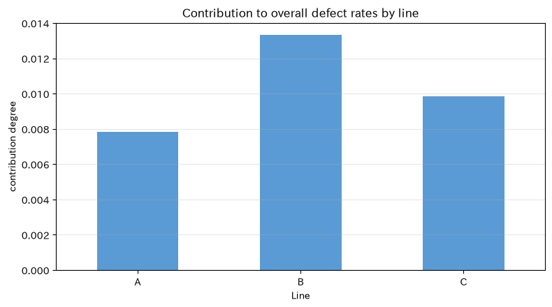
Total contribution = 3.10%
Direct Aggregate P(D) = 3.10%

Reading the results

The total contribution matches the overall defect rate directly aggregated. Improvement priorities should be determined not only by the defect rate on the line, but also by contribution by multiplying the production composition ratio, potential for improvement, and loss unit cost.

No.009: Bayes’ Theorem

Meaning in Practice

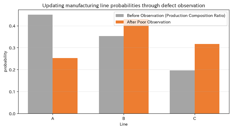
When one defective product is found, update which line is most likely to come from. The line with the highest defect rate and the line with the highest total defect generation may not match due to differences in production volume.

Approach to Analysis and Modeling

The probability of line $L_i$ after observing defective products is,

$P(L_i\mid D)=\frac{P(D\mid L_i)P(L_i)}{P(D)}$

That’s right. $P(L_i)$ is the prior probability (production composition ratio), $P(D\mid L_i)$ is the likelihood, and $P(L_i\mid D)$ is the posterior probability. The molecule matches the contribution level of No.008.

Check with Python

bayes = line_stats[["Production Composition Ratio", "Line Defect Rate", "Contribution to the overall defect rate"]].copy()
bayes["Line Probability After Poor Observation"] = bayes["Contribution to the overall defect rate"] / p_D
bayes["Direct aggregation from defective products"] = df.loc[df["is_defect"], "line"].value_counts(normalize=True).sort_index()
display(bayes.style.format("{:.2%}"))

x = np.arange(len(bayes))
width = 0.35
plt.bar(x - width/2, bayes["Production Composition Ratio"], width, label="Before Observation (Production Composition Ratio)", color="#A5A5A5")
plt.bar(x + width/2, bayes["Line Probability After Poor Observation"], width, label="After Poor Observation", color="#ED7D31")
plt.title("Updating manufacturing line probabilities through defect observation")
plt.xlabel("Line")
plt.ylabel("probability")
plt.xticks(x, bayes.index)
plt.legend()
plt.grid(axis="y", alpha=0.3)
plt.tight_layout()
plt.show()

	Production Composition Ratio	Line Defect Rate	Contribution to the overall defect rate	Line Probability After Poor Observation	Direct aggregation from defective products
line
A	45.03%	1.74%	0.78%	25.27%	25.27%
B	35.30%	3.78%	1.33%	43.01%	43.01%
C	19.67%	5.00%	0.98%	31.72%	31.72%

Reading the results

After defect detection, the probability of lines with high defect rates increases compared to the production composition ratio. Bayes’ theorem is not a formula for determining causes, but rather a formula that rationally updates the order of investigations by integrating pre-observation composition ratios and likelihood under various conditions.

No.010: Monte Carlo Method and the Law of Large Numbers

Meaning in Practice

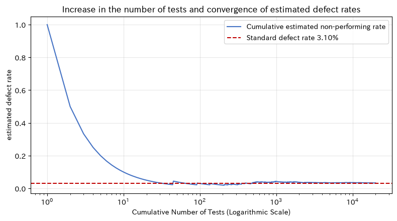
For a small number of spot checks, the preliminary defect rate can fluctuate significantly. By simulating how stable the estimates are when the number of tests increases, you can discuss how to handle preliminary values, test costs, and the required sample size.

Approach to Analysis and Modeling

The mean of the Bernoulli variable $X_i\in\{0,1\}$ that follows the same distribution independently

$\bar{X}_n=\frac{1}{n}\sum_{i=1}^n X_i$

As the $n$ increases, it approaches the true defect probability $p$. This is the law of large numbers. In the Monte Carlo method, repeated trials using random numbers are performed to numerically identify variations in estimates and judgment errors.

Check with Python

true_rate = p_D
mc_rng = np.random.default_rng(SEED + 1)
sample_sizes = [20, 50, 100, 500, 2_000]
n_repeats = 2_000

mc_rows = []
for n in sample_sizes:
    estimates = mc_rng.binomial(n, true_rate, size=n_repeats) / n
    mc_rows.append({
        "number_of_inspections n": n,
        "Average estimated defect rate": estimates.mean(),
        "standard_deviation": estimates.std(ddof=1),
        "mean absolute error": np.mean(np.abs(estimates - true_rate)),
    })
mc_summary = pd.DataFrame(mc_rows)
display(mc_summary.style.format({
    "Average estimated defect rate": "{:.3%}", "standard_deviation": "{:.3%}", "mean absolute error": "{:.3%}"
}))

stream = mc_rng.random(20_000) < true_rate
running_rate = np.cumsum(stream) / np.arange(1, len(stream) + 1)
plt.plot(np.arange(1, len(stream) + 1), running_rate, label="Cumulative estimated non-performing rate", color="#4472C4")
plt.axhline(true_rate, color="#C00000", linestyle="--", label=f"Standard defect rate {true_rate:.2%}")
plt.xscale("log")
plt.title("Increase in the number of tests and convergence of estimated defect rates")
plt.xlabel("Cumulative Number of Tests (Logarithmic Scale)")
plt.ylabel("estimated defect rate")
plt.legend()
plt.grid(True, alpha=0.3)
plt.tight_layout()
plt.show()

	number_of_inspections n	Average estimated defect rate	standard_deviation	mean absolute error
0	20	3.143%	3.962%	3.366%
1	50	3.070%	2.393%	1.984%
2	100	3.066%	1.761%	1.378%
3	500	3.094%	0.767%	0.610%
4	2000	3.117%	0.389%	0.307%

Reading the results

In iterative simulation, the more tests are used, the smaller the standard deviation and mean absolute error of the estimate. The cumulative defect rate fluctuates significantly at first, but gradually stabilizes near the reference value. Since the law of large numbers does not guarantee that even small numbers are correct, preliminary values should include both denominators and uncertainty.

Practical Implications Seen Through Target Exercise

1. Definitions determine analysis quality: If you do not fix the sample space, events, periods, and exclusion criteria at first, even with correct calculations, comparisons will be incomparable.
2. The overall value is broken down into structure.: Using the total probability theorem, separating the composition ratio and conditional defect rate can explain whether the deterioration is due to production transfer or in-process changes.
3. Prioritize the cause candidates to update Bayes’ priorities.: The order of investigations is determined not only by high defect rates but also by their contribution to the overall defective product, including production volume.
4. Independence is not a hypothesis, but a subject of verification: When setting up independence for simplification, clearly state its impact and diagnostic results.
5. Preliminary values for small samples vary widely.: Instead of issuing alerts based solely on point estimation, design sample size, control limits, and false alarm costs.

What is necessary for practical implementation

• product_id data model that can track equipment, lines, shifts, times, and inspection results
• Definitions of defects, reinspection, rework, and disposal, as well as rules for handling missing measurements, duplicates, and re-measurements
• A dashboard that simultaneously displays conditional defect rates and production composition ratios by line
• Data quality testing to detect sharp denominator reductions and total classification discrepancies
• Alert criteria separating statistical differences from practical differences warranting suspension or adjustment
• Responsible Person and Operational Procedures Connecting Cause Investigation, Countermeasure Implementation, and Effectiveness Verification

Improvement is not achieved by probability calculations alone. It can only be used for decision-making when combined with on-site knowledge, measurement systems, loss amounts, and countermeasures.

Conclusion

From No.001 to No.010, manufacturing quality data was used to check everything from sets to the law of large numbers in a single flow. The important thing is not to rush to give the answer of the overall defect rate, but to be able to explain the What denominators were used, what conditions were assigned, which assumptions were used for calculation, and how sample variation was handled..

In the next analysis, by stacking probability distributions, expected values and variances, statistical estimates, and hypothesis testing on this foundation, we can quantify improvement effects and future risks.

Consultations for Corporations

At Suri Kobo, we support data analysis, PoC design, and in-house training related to quality control, anomaly detection, demand forecasting, and mathematical optimization in manufacturing. From defining on-site KPIs to the analysis foundation and implementation into decision-making processes, we organize everything according to each issue.

📩 Contact Us: surikobo.co.jp/contact
Please feel free to consult us first.