100 Exercises / Probability Statistics / 100 Exercises on Probability and Statistical Theory

Reading Multiple KPIs Simultaneously—Multivariate Probabilities of Manufacturing Quality, Equipment Load, and Delivery Risks

2020-04-14

Reading Multiple KPIs Simultaneously—Multivariate Probabilities of Manufacturing Quality, Equipment Load, and Delivery Risks

Overview

In manufacturing sites, temperature, pressure, dimensions, roughness, and power fluctuate simultaneously. If you only follow the average of individual KPIs, you may overlook quality risks that arise in combinations and predicted changes after adding conditions. This article uses data from 900 lots of a fictional precision molding factory to connect Simultaneous distribution, peripheral distribution, conditional distribution, independence, covariance matrix, correlation matrix, multivariate normal distribution, conditional normal distribution, Gaussian process, copula to process monitoring and decision-making.

The subject is the No.061〜No.070 of ‘100 Exercises on Probability and Statistical Theory.’ Instead of stopping at mere calculations for each method, we connect to practical questions such as “Which combinations of conditions should we monitor?”, “How can additional information change predictions?”, and “How much capacity do we have to withstand simultaneous risk?”

[!NOTE] This material is a notebook previously used by Surikoubo (or personally by the representative, Kazuyama), and has been reconstructed, edited, and published with the company’s permission.
All data listed is fictional and has no relation whatsoever to real companies, factories, or figures.

Introduction: Practical Challenges in Manufacturing Covered in This Article

The subject is a precision molding factory that produces products A, B, and C using common equipment. Administrators are required to make the following decisions.

Can you capture lots where both dimensional and surface roughness deteriorate faster than a standalone KPI?
How to update the probability of quality status when the temperature range is known.
Are these two abnormalities just a coincidence, or are there dependencies?
Managing multiple sensors in a matrix to detect redundant indicators and linkage directions
Can the power intensity after temperature observation be predicted by distribution rather than points?
Can equipment drift, which changes smoothly over time, be interpolated with uncertainty?
Can only simultaneous risks be represented without changing the peripheral distribution of downtime and delivery time losses?

The role of multivariate probability is not to “increase the number of columns.” It involves translating the probability structures created by multiple KPIs into monitoring rules, maintenance plans, quality assurance, and BCP decisions.

Common situations on site

Dimensions and roughness are monitored separately on separate control charts, and both are slightly less reliable for lots that are missed
The overall defect rate is reported, but the probability of occurrence under conditions such as high temperatures or night shifts is not indicated
Interpreting a correlation close to zero as “independence”
The covariance matrix dominated by variables with large units is used directly to compare the strength of the relation
Mechanically applying a multivariate normal distribution to all data without checking the distribution shape
Only look at interpolation curves and ignore uncertainty in unobserved intervals
Generate random numbers independently for downtime and loss amounts, and underestimate simultaneous tail risk.

In all cases, the problem lies more in the misunderstanding between assumptions and applications than the calculations themselves. In this article, we will clarify which questions the model can answer and which cannot by going back and forth between tables, formulas, and diagrams.

Why is this issue so difficult to judge?

Having only two variables does not determine the probability by the “distribution of each individual” alone. Even if the peripheral distributions of $X$ and $Y$ are the same, there can be multiple simultaneous distributions $p(x,y)$ . Different dependency structures also affect the probability of simultaneous anomalies and total losses.

Also, when conditions are added, the evaluation targets change. The overall probability $P(Y)$ and the $P(Y\mid X)$ after determining the temperature range are different things. The latter is a prediction based on information observable on site, but if the conditions are too fine, the number of relevant lots decreases, making the estimate unstable.

Furthermore, the normal distribution, Gaussian process, and copula are all related to the word “Gauss,” but their roles differ. Multivariate normal distribution deals with simultaneous vectors, conditional normal distribution deals with post-observation updates, Gaussian processes cover the set of functions, and Gausscopulars deal with the separation of peripheral distribution and dependent structure.

Overview of Exercise covered this time

No.	Theme	Questions in the Manufacturing Industry
061	simultaneous distribution	What percentage is the combination of dimensional and roughness conditions?
062	peripheral distribution	Can you extract the individual KPI distributions from simultaneous tables?
063	Conditional distribution	How does knowing the temperature zone change the probability of roughness states?
064	independence	Can high temperature and abnormal roughness be considered independent?
065	codisperse matrix	Can you express variation and co-fluctuation across multiple KPIs in one place?
066	correlation matrix	Can you compare the strength of relationships except for units?
067	multivariate normal distribution	Can the normal areas of multiple KPIs be captured as ellipses?
068	Conditional normal distribution	Can the power distribution after temperature observation be updated?
069	Gaussian process	Can equipment drift be interpolated with uncertainty?
070	Copula	Can it represent the simultaneous risk of irregular downtime and loss?

From No.061 to No.064, we move on to the basics of probability tables; from No.065 to No.068, we move on to vector distributions; and from No.069 to No.070, we move on to models of functions and dependency structures.

Preparing the Python environment

NumPy handles random number and matrix calculations, pandas aggregates, matplotlib visualization, and SciPy handles quantiles of normal distributions. It does not depend on external data or seaborn. Fix the random seed so that the result is the same after rerunting.

import platform
import sys

import japanize_matplotlib  # noqa: F401 Japanese font settings
import matplotlib
import matplotlib.pyplot as plt
import numpy as np
import pandas as pd
from IPython.display import display
from scipy.stats import chi2, norm

SEED = 20260711
rng = np.random.default_rng(SEED)

pd.set_option("display.max_columns", 30)
pd.set_option("display.float_format", lambda x: f"{x:,.4f}")
plt.rcParams["figure.figsize"] = (8, 4.8)
plt.rcParams["axes.unicode_minus"] = False

print(f"Python: {sys.version.split()[0]}")
print(f"OS: {platform.system()} {platform.release()}")
print(f"NumPy: {np.__version__}")
print(f"pandas: {pd.__version__}")
print(f"matplotlib: {matplotlib.__version__}")
print(f"random number seed: {SEED}")

Python: 3.11.9
OS: Darwin 25.3.0
NumPy: 1.26.4
pandas: 2.2.2
matplotlib: 3.9.2
Random number seed: 20260711

Creation of Fictional Data

For 900 lots, we generate the product, working zone, mold temperature, injection pressure, dimensional deviation, surface roughness, and power intensity. We reflect common latent fluctuations in multiple KPIs and simulate the interactions occurring on site.

On the high-temperature side, dimensional deviations, roughness, and power consumption tend to increase more easily.
Pressure rise works to suppress dimensional deviations and roughness.
Average levels differ slightly depending on product and work period
Standard determination is set as dimensional deviation of $\pm 0.030$ mm and surface roughness of $1.05\ \mu$ m or less

This is not data for estimating causal effects, but rather fictitious data to confirm the behavior of multivariate probabilities.

n = 900
product = rng.choice(["ProductsA", "ProductsB", "ProductsC"], n, p=[0.45, 0.35, 0.20])
shift = rng.choice(["day shift", "night shift"], n, p=[0.68, 0.32])
night = (shift == "night shift").astype(float)
product_temp = pd.Series(product).map({"ProductsA": 0.0, "ProductsB": 1.3, "ProductsC": -0.8}).to_numpy()
product_pressure = pd.Series(product).map({"ProductsA": 0.0, "ProductsB": 2.2, "ProductsC": -1.5}).to_numpy()
product_dimension = pd.Series(product).map({"ProductsA": 0.000, "ProductsB": 0.004, "ProductsC": -0.003}).to_numpy()
product_roughness = pd.Series(product).map({"ProductsA": 0.00, "ProductsB": 0.07, "ProductsC": 0.12}).to_numpy()
product_energy = pd.Series(product).map({"ProductsA": 0.00, "ProductsB": 0.10, "ProductsC": 0.18}).to_numpy()

z1, z2, z3, z4, z5 = rng.normal(size=(5, n))
temp_std = z1
pressure_std = 0.25 * z1 + np.sqrt(1 - 0.25**2) * z2
dimension_std = 0.55 * z1 - 0.30 * z2 + np.sqrt(1 - 0.55**2 - 0.30**2) * z3
roughness_std = 0.40 * z1 - 0.25 * z2 + 0.55 * z3 + np.sqrt(1 - 0.40**2 - 0.25**2 - 0.55**2) * z4
energy_std = 0.65 * z1 + 0.20 * z2 + np.sqrt(1 - 0.65**2 - 0.20**2) * z5

mold_temp = 180 + product_temp + 1.4 * night + 4.2 * temp_std
injection_pressure = 92 + product_pressure + 1.0 * night + 5.5 * pressure_std
dimension_deviation = product_dimension + 0.002 * night + 0.018 * dimension_std
surface_roughness = product_roughness + 0.035 * night + 0.76 + 0.20 * roughness_std
energy_kwh = product_energy + 0.05 * night + 1.85 + 0.24 * energy_std

df = pd.DataFrame({
    "lotID": [f"L{i:04d}" for i in range(1, n + 1)],
    "Products": product,
    "Work Schedule": shift,
    "mold_temperature_c": mold_temp,
    "injection_pressure_mpa": injection_pressure,
    "dimensional_deviation_mm": dimension_deviation,
    "surface_roughness_um": surface_roughness,
    "electricity_intensity_kwh": energy_kwh,
})
df["Dimensional condition"] = pd.cut(
    df["dimensional_deviation_mm"], [-np.inf, -0.030, 0.030, np.inf],
    labels=["Outside the lower limit", "Within the standard", "outside the upper limit"]
)
df["roughness condition"] = np.where(df["surface_roughness_um"] <= 1.05, "Within the standard", "Outside the standard")
df["temperature zone"] = pd.cut(
    df["mold_temperature_c"], [-np.inf, 178, 184, np.inf],
    labels=["low temperature", "Standard", "high temperature"]
)
df["Overall Judgment"] = np.where(
    (df["Dimensional condition"] == "Within the standard") & (df["roughness condition"] == "Within the standard"), "qualified", "Needs confirmation"
)

display(df.head(8).round(4))
display(
    df.groupby("Products", observed=True).agg(
        lot_size=("lotID", "size"),
        average_temperature_c=("mold_temperature_c", "mean"),
        average_dimensional_deviation_mm=("dimensional_deviation_mm", "mean"),
        average_roughness_um=("surface_roughness_um", "mean"),
        confirmation_rate=("Overall Judgment", lambda s: (s == "Needs confirmation").mean()),
    ).round(4)
)
print(f"Number of missing items: {int(df.isna().sum().sum())} / Total number of cells: {df.size:,}")

	lotID	Products	Work Schedule	mold_temperature_C	injection_pressure_MPa	dimensional_deviation_mm	surface_roughness_um	electricity_intensity_kWh	Dimensional condition	roughness condition	temperature zone	Overall Judgment
0	L0001	ProductsA	day shift	188.8566	93.2255	0.0261	1.0195	2.0346	Within the standard	Within the standard	high temperature	qualified
1	L0002	ProductsC	day shift	175.9133	88.3551	-0.0191	0.8189	1.9327	Within the standard	Within the standard	low temperature	qualified
2	L0003	ProductsB	night shift	183.1683	95.6314	0.0003	0.6809	1.9350	Within the standard	Within the standard	Standard	qualified
3	L0004	ProductsB	day shift	179.5093	95.3241	-0.0115	0.5540	1.5872	Within the standard	Within the standard	Standard	qualified
4	L0005	ProductsC	day shift	174.6242	88.3919	-0.0006	0.6642	1.7433	Within the standard	Within the standard	low temperature	qualified
5	L0006	ProductsA	night shift	184.7163	90.1155	-0.0029	0.7349	2.2325	Within the standard	Within the standard	high temperature	qualified
6	L0007	ProductsA	day shift	180.6574	92.1942	-0.0207	0.6606	2.2577	Within the standard	Within the standard	Standard	qualified
7	L0008	ProductsC	day shift	182.1593	87.6065	-0.0066	0.9197	2.0499	Within the standard	Within the standard	Standard	qualified

	lot_size	average temperature_C	Average dimensional deviation_mm	Average roughness_um	confirmation_rate
Products
ProductsA	415	180.2865	0.0010	0.7668	0.1446
ProductsB	321	181.7583	0.0037	0.8398	0.1838
ProductsC	164	179.2849	-0.0015	0.8972	0.2683

Number of Missing Cells: 0 / Total Cells: 10,800

No.061: Simultaneous Distribution

Meaning in Practice

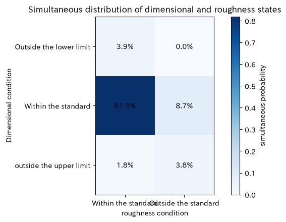
Simply looking at dimensions and roughness separately does not reveal combination risks such as “not above the upper limit of dimensions and outside the standard roughness.” Simultaneous distribution represents the probability that multiple quality states At the same time occur and can be used for designing composite judgments and sorting capabilities.

Approach to Analysis and Modeling

The simultaneous probability mass function of discrete variable $X,Y$ is

p_{X,Y}(x,y)=P(X=x,Y=y), \qquad \sum_x\sum_y p_{X,Y}(x,y)=1

That’s right. For the data, we use the experience simultaneity probability, which is the number of lots for each combination divided by the total 900 lots. Including 0 combinations, confirm that the total in the probability table is 1.

Check with Python

dimension_order = ["Outside the lower limit", "Within the standard", "outside the upper limit"]
roughness_order = ["Within the standard", "Outside the standard"]
joint_count = pd.crosstab(df["Dimensional condition"], df["roughness condition"]).reindex(
    index=dimension_order, columns=roughness_order, fill_value=0
)
joint_prob = joint_count / len(df)
display(joint_count.rename_axis("Dimensional condition / lot_size"))
display(joint_prob.rename_axis("Dimensional condition / simultaneous probability").round(4))
print(f"sum of simultaneous probabilities: {joint_prob.to_numpy().sum():.6f}")

fig, ax = plt.subplots(figsize=(7, 4.5))
im = ax.imshow(joint_prob.to_numpy(), cmap="Blues", vmin=0)
ax.set_xticks(range(len(roughness_order)), roughness_order)
ax.set_yticks(range(len(dimension_order)), dimension_order)
for i in range(len(dimension_order)):
    for j in range(len(roughness_order)):
        ax.text(j, i, f"{joint_prob.iloc[i, j]:.1%}", ha="center", va="center")
fig.colorbar(im, ax=ax, label="simultaneous probability")
ax.set_title("Simultaneous distribution of dimensional and roughness states")
ax.set_xlabel("roughness condition")
ax.set_ylabel("Dimensional condition")
ax.grid(False)
plt.tight_layout()
plt.show()

roughness condition	Within the standard	Outside the standard
Dimensional condition / lot_size
Outside the lower limit	35	0
Within the standard	737	78
outside the upper limit	16	34

roughness condition	Within the standard	Outside the standard
Dimensional condition / simultaneous probability
Outside the lower limit	0.0389	0.0000
Within the standard	0.8189	0.0867
outside the upper limit	0.0178	0.0378

Total simultaneous probability: 1.000000

png

Reading the results

One cell in the probability table shows the simultaneous occurrence rate of two states. Even if the number of within standard × specification is the largest, the scale of the selection target can be determined by summing the combined confirmation cells. In practice, this table is compared by product, equipment, and period, and cells with fewer cases show not only the rate but also the actual number. Since the boundaries of standard judgments change as the simultaneous distribution changes, judgment definitions and version management are necessary.

No.062: Peripheral Distribution

Meaning in Practice

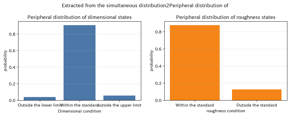
The peripheral distribution is the sum of the other person’s states from the simultaneous distribution, and the distribution of only dimensions and roughness is extracted. You can verify whether the overall quality KPI and the composite judgment table are consistent.

Approach to Analysis and Modeling

The peripheral distribution of $X$ obtained by summing $Y$ is

p_X(x)=\sum_y p_{X,Y}(x,y)

and similarly, $p_Y(y)=\sum_x p_{X,Y}(x,y)$ . “Periphery” comes from the fact that the sum is placed at the end of the row or column in the simultaneous probability table. From the peripheral distribution alone, you cannot reconstruct how the two variables combine.

Check with Python

margin_dimension = joint_prob.sum(axis=1).rename("Probability around dimensions from simultaneous tables")
margin_roughness = joint_prob.sum(axis=0).rename("Roughness Marginal Probabilities from Simultaneous Tables")
direct_dimension = df["Dimensional condition"].value_counts(normalize=True).reindex(dimension_order).rename("direct aggregation")
direct_roughness = df["roughness condition"].value_counts(normalize=True).reindex(roughness_order).rename("direct aggregation")

display(pd.concat([margin_dimension, direct_dimension], axis=1).round(4))
display(pd.concat([margin_roughness, direct_roughness], axis=1).round(4))

fig, axes = plt.subplots(1, 2, figsize=(10, 4))
axes[0].bar(margin_dimension.index, margin_dimension.values, color="#4C78A8")
axes[0].set_title("Peripheral distribution of dimensional states")
axes[0].set_xlabel("Dimensional condition")
axes[0].set_ylabel("probability")
axes[0].grid(axis="y", alpha=0.3)
axes[1].bar(margin_roughness.index, margin_roughness.values, color="#F58518")
axes[1].set_title("Peripheral distribution of roughness states")
axes[1].set_xlabel("roughness condition")
axes[1].set_ylabel("probability")
axes[1].grid(axis="y", alpha=0.3)
fig.suptitle("Extracted from the simultaneous distribution2Peripheral distribution of")
plt.tight_layout()
plt.show()

	Probability around dimensions from simultaneous tables	direct aggregation
Dimensional condition
Outside the lower limit	0.0389	0.0389
Within the standard	0.9056	0.9056
outside the upper limit	0.0556	0.0556

	Roughness Marginal Probabilities from Simultaneous Tables	direct aggregation
roughness condition
Within the standard	0.8756	0.8756
Outside the standard	0.1244	0.1244

png

Reading the results

The row and column sums in the simultaneous probability table match the probabilities of the original data aggregated alone. However, for example, based only on peripheral KPIs like roughness non-standard rate, it is not possible to determine whether the lot was within the dimensional specifications. Management reports should keep peripheral KPIs concise, but for selection, cause analysis, and composite assurance, keeping simultaneous distributions is necessary.

No.063: Conditional Distribution

Meaning in Practice

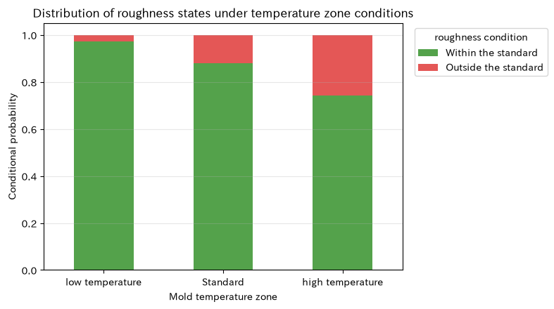
After the mold temperature zone is observed, the probability of the roughness state is updated. Since it shows the “percentage at high temperature” rather than the overall defect rate, it serves as a basis for strengthening extraction and adjusting conditions after temperature alarms.

Approach to Analysis and Modeling

$P(X=x)>0$ , the conditional probability is

P(Y=y\mid X=x)=\frac{P(X=x,Y=y)}{P(X=x)}

That’s right. Normalize the total within rows in each temperature zone to be 1. Differences in conditional distribution indicate correlation but do not directly indicate the causal effect of temperature manipulation. Product configurations and work schedules may be mixed.

Check with Python

temp_order = ["low temperature", "Standard", "high temperature"]
conditional_count = pd.crosstab(df["temperature zone"], df["roughness condition"]).reindex(
    index=temp_order, columns=roughness_order, fill_value=0
)
conditional_prob = conditional_count.div(conditional_count.sum(axis=1), axis=0)
display(conditional_count.rename_axis("temperature zone / lot_size"))
display(conditional_prob.rename_axis("temperature zone / Conditional probability").round(4))
print("Total probability by temperature zone:")
display(conditional_prob.sum(axis=1).rename("Total").to_frame())

conditional_prob.plot(kind="bar", stacked=True, color=["#54A24B", "#E45756"], figsize=(8, 4.5))
plt.title("Distribution of roughness states under temperature zone conditions")
plt.xlabel("Mold temperature zone")
plt.ylabel("Conditional probability")
plt.xticks(rotation=0)
plt.grid(axis="y", alpha=0.3)
plt.legend(title="roughness condition", bbox_to_anchor=(1.02, 1), loc="upper left")
plt.tight_layout()
plt.show()

roughness condition	Within the standard	Outside the standard
temperature zone / lot_size
low temperature	253	7
Standard	382	52
high temperature	153	53

roughness condition	Within the standard	Outside the standard
temperature zone / Conditional probability
low temperature	0.9731	0.0269
Standard	0.8802	0.1198
high temperature	0.7427	0.2573

Total probability at each temperature range:

	Total
temperature zone
low temperature	1.0000
Standard	1.0000
high temperature	1.0000

png

Reading the results

The ratio of non-standard roughness varies by temperature range, showing that temperature information can be used to update quality probabilities. In alarm design, not only the non-standard rate but also the lot count for each band, false alarm costs, and missed incident costs are also recorded. If the high-temperature zone is too narrow, the number of relevant cases decreases, so thresholds are determined based on physical knowledge and the required detection power.

No.064: Independence

Meaning in Practice

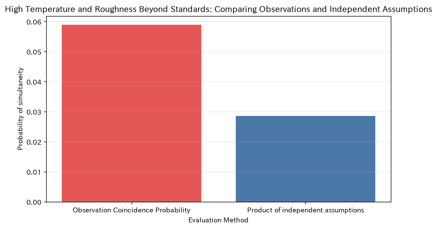
If high temperature and non-standard coarsity are separate, the simultaneous generation rate is estimated by the product of each rate. FMEA and simulations, which are not independent and only multiply individual risks, underestimate or overestimate simultaneous anomalies.

Approach to Analysis and Modeling

$X,Y$ is said to be independent in all combinations

P(X=x,Y=y)=P(X=x)P(Y=y)

This is what holds true. This time, we will compare the simultaneous observation probability and the product under independent assumptions for two events: “high temperature” and “abnormal roughness.” Since a finite sample does not match perfectly, we examine the magnitude of the difference, operational impact, and period stability. A correlation of 0 generally does not guarantee independence.

Check with Python

is_high_temp = df["temperature zone"].eq("high temperature")
is_rough_ng = df["roughness condition"].eq("Outside the standard")
p_high = is_high_temp.mean()
p_ng = is_rough_ng.mean()
p_both = (is_high_temp & is_rough_ng).mean()
p_product = p_high * p_ng

independence_table = pd.DataFrame({
    "indicator": ["P(high temperature)", "P(Roughness Beyond Standard)", "Observation P(high temperature∩Roughness Beyond Standard)", "Independent assumption P(high temperature)P(Roughness Beyond Standard)"],
    "probability": [p_high, p_ng, p_both, p_product],
})
display(independence_table.assign(probability_pct=lambda x: x["probability"].map(lambda v: f"{v:.2%}")))
print(f"Simultaneous Probability Ratio (Observation / Independent Assumption): {p_both / p_product:.2f} double")
print(f"Guideline for additional concurrent lot sizes: {(p_both - p_product) * len(df):.1f} lot / {len(df)}lot")

plt.bar(["Observation Coincidence Probability", "Product of independent assumptions"], [p_both, p_product], color=["#E45756", "#4C78A8"])
plt.title("High Temperature and Roughness Beyond Standards: Comparing Observations and Independent Assumptions")
plt.xlabel("Evaluation Method")
plt.ylabel("Probability of simultaneity")
plt.grid(axis="y", alpha=0.3)
plt.tight_layout()
plt.show()

	indicator	probability	probability_pct
0	P(high temperature)	0.2289	22.89%
1	P(Roughness Beyond Standard)	0.1244	12.44%
2	Observation P(high temperature∩Roughness Beyond Standard)	0.0589	5.89%
3	Independent assumption P(high temperature)P(Roughness Beyond Standard)	0.0285	2.85%

Simultaneous Probability Ratio (Observation / Independent Assumption): 2.07 times
Estimated additional concurrent lots: 27.4 lots / 900 lots

png

Reading the results

If the probability of observation concurrency exceeds the product of the independent assumptions, a risk model that independently generates two events underestimates the simultaneity. However, this is not an independence test for all combinations of values. In practical implementation, we check the expected frequency of cross-tabulation, stratification by product and work period, and reproducibility across multiple periods, and use chi-square tests and regression models as supplementary measures as needed.

No.065: Covariance Matrix

Meaning in Practice

As the number of sensors increases, it becomes difficult to individually manage covariance between two variables. The covariance matrix consolidates the variation and covariation between KPIs into a single symmetric matrix, serving as the basis for risk calculation and multivariate monitoring of linear composite KPIs.

Approach to Analysis and Modeling

The covariance matrix of a probability vector $\mathbf{X}=(X_1,\ldots,X_p)^\top$ is

\boldsymbol{\Sigma}=E[(\mathbf{X}-\boldsymbol{\mu})(\mathbf{X}-\boldsymbol{\mu})^\top]

That’s right. The diagonal component is dispersed, the non-diagonal component is covariance, and $\Sigma_{ij}=\Sigma_{ji}$ . For any weight $\mathbf{a}$ , $\mathrm{Var}(\mathbf{a}^\top\mathbf{X})=\mathbf{a}^\top\boldsymbol{\Sigma}\mathbf{a}$ is the value.

Check with Python

sensor_cols = ["mold_temperature_c", "injection_pressure_mpa", "dimensional_deviation_mm", "surface_roughness_um", "electricity_intensity_kwh"]
cov_matrix = df[sensor_cols].cov()
display(cov_matrix.round(6))
print(f"Maximum error in symmetry: {np.abs(cov_matrix.to_numpy() - cov_matrix.to_numpy().T).max():.2e}")
print(f"Minimum eigenvalue: {np.linalg.eigvalsh(cov_matrix.to_numpy()).min():.8f}（0If that's the case, then semi-positive definite values)")

# Normalizing temperature and pressure and confirming the dispersion of process load indices synthesized under the same weight
two = df[["mold_temperature_c", "injection_pressure_mpa"]]
two_z = (two - two.mean()) / two.std(ddof=1)
sigma_two = two_z.cov().to_numpy()
a = np.array([0.6, 0.4])
load_index = two_z.to_numpy() @ a
var_matrix = a @ sigma_two @ a
var_direct = load_index.var(ddof=1)
display(pd.DataFrame({"Calculation method": ["a'Σa", "Direct calculation after synthesis"], "disperse": [var_matrix, var_direct]}).round(6))

fig, ax = plt.subplots(figsize=(8, 6))
im = ax.imshow(cov_matrix.to_numpy(), cmap="RdBu_r")
ax.set_xticks(range(len(sensor_cols)), sensor_cols, rotation=30, ha="right")
ax.set_yticks(range(len(sensor_cols)), sensor_cols)
fig.colorbar(im, ax=ax, label="covariance (unit-dependent)")
ax.set_title("ProjectKPICovariance matrix")
ax.set_xlabel("KPI")
ax.set_ylabel("KPI")
ax.grid(False)
plt.tight_layout()
plt.show()

	mold_temperature_C	injection_pressure_MPa	dimensional_deviation_mm	surface_roughness_um	electricity_intensity_kWh
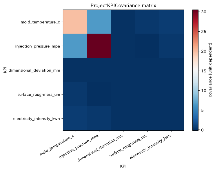
mold_temperature_C	19.8177	6.5382	0.0462	0.3915	0.6696
injection_pressure_MPa	6.5382	30.4943	-0.0136	-0.1519	0.4433
dimensional_deviation_mm	0.0462	-0.0136	0.0003	0.0027	0.0013
surface_roughness_um	0.3915	-0.1519	0.0027	0.0421	0.0151
electricity_intensity_kWh	0.6696	0.4433	0.0013	0.0151	0.0606

Maximum error of symmetry: 0.00e+00
Minimum eigenvalue: 0.00012796 (0 or higher is a semidefinite)

	Calculation method	disperse
0	a'Σa	0.6477
1	Direct calculation after synthesis	0.6477

png

Reading the results

The covariance matrix is symmetrical, with the variance of each indicator arranged diagonally. Also, the variance of the composite index calculated by the determinant matches the direct calculation. On the other hand, since millimeters and MPa differ greatly in units and scales, you cannot compare the strength of the relationship solely by the size of the color. For calculating loss variance without the unit intensity, covariance is used; for comparing relationships, the following correlation matrix is used.

No.066: Correlation Matrix

Meaning in Practice

The correlation matrix standardizes each KPI and compares the direction and strength of linear relationships from $-1$ to $1$ . Sensors with similar information, candidate conditions linked to quality, and gateways to explore the possibility of multicollinearity.

Approach to Analysis and Modeling

Let the diagonal matrix of standard deviations be $\mathbf{D}$ , then the correlation matrix is

\mathbf{R}=\mathbf{D}^{-1}\boldsymbol{\Sigma}\mathbf{D}^{-1}

That’s right. The diagonal component is 1 and is not affected by unit conversion. However, Pearson correlation is an indicator of linear relationships, so caution is needed regarding nonlinear relationships, outliers, and group mixing. Correlation does not imply causation.

Check with Python

std = df[sensor_cols].std(ddof=1).to_numpy()
d_inv = np.diag(1 / std)
corr_from_cov = d_inv @ cov_matrix.to_numpy() @ d_inv
corr_direct = df[sensor_cols].corr().to_numpy()
correlation = pd.DataFrame(corr_direct, index=sensor_cols, columns=sensor_cols)
display(correlation.round(3))
print(f"Maximum difference from calculations from the covariance matrix: {np.abs(corr_from_cov - corr_direct).max():.2e}")

fig, ax = plt.subplots(figsize=(8, 6))
im = ax.imshow(corr_direct, vmin=-1, vmax=1, cmap="RdBu_r")
ax.set_xticks(range(len(sensor_cols)), sensor_cols, rotation=30, ha="right")
ax.set_yticks(range(len(sensor_cols)), sensor_cols)
for i in range(len(sensor_cols)):
    for j in range(len(sensor_cols)):
        ax.text(j, i, f"{corr_direct[i, j]:.2f}", ha="center", va="center",
                color="white" if abs(corr_direct[i, j]) > 0.55 else "black")
fig.colorbar(im, ax=ax, label="Pearsoncorrelation coefficient")
ax.set_title("ProjectKPICorrelation matrix")
ax.set_xlabel("KPI")
ax.set_ylabel("KPI")
ax.grid(False)
plt.tight_layout()
plt.show()

	mold_temperature_C	injection_pressure_MPa	dimensional_deviation_mm	surface_roughness_um	electricity_intensity_kWh
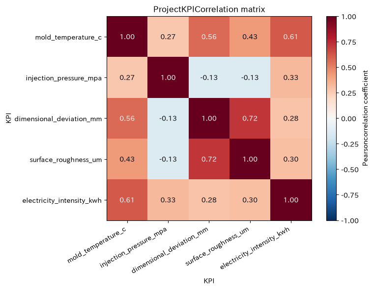
mold_temperature_C	1.0000	0.2660	0.5650	0.4290	0.6110
injection_pressure_MPa	0.2660	1.0000	-0.1340	-0.1340	0.3260
dimensional_deviation_mm	0.5650	-0.1340	1.0000	0.7150	0.2850
surface_roughness_um	0.4290	-0.1340	0.7150	1.0000	0.2980
electricity_intensity_kWh	0.6110	0.3260	0.2850	0.2980	1.0000

Maximum difference from calculation from the covariance matrix: 1.94e-15

png

Reading the results

You can compare positive and negative correlations such as dimensional deviations, roughness, and temperature regardless of the unit. Sensors with strong correlations can provide clues for redundancy or potential causes, but removing one does not necessarily mean you can remove one. Control response speed, calibration methods, and failure modes are also taken into account. Since product-specific correlation and overall correlation can be reversed, equipment conditions are not changed only in the global matrix.

No.067: Multivariate Normal Distribution

Meaning in Practice

Even if individual KPIs fall within control limits, combinations may fall outside the usual range. The multivariate normal distribution represents an elliptical normal region with mean vectors and covariance matrices, and can be used for simultaneous monitoring of multiple sensors and for anomalous candidate extraction.

Approach to Analysis and Modeling

$p$ The density of the dimensional multivariate normal distribution is

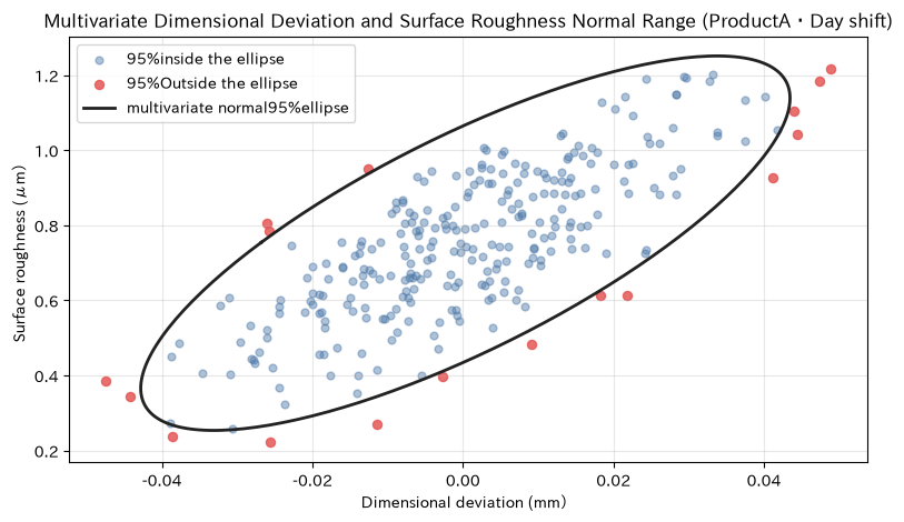
f(\mathbf{x})=\frac{1}{(2\pi)^{p/2}|\boldsymbol{\Sigma}|^{1/2}} \exp\left[-\frac{1}{2}(\mathbf{x}-\boldsymbol{\mu})^\top \boldsymbol{\Sigma}^{-1}(\mathbf{x}-\boldsymbol{\mu})\right]

That’s right. The secondary form of the exponent part is the square $D_M^2$ of the Mahalanobis distance. Under the normal assumption, $D_M^2$ generally follows a chi-square distribution with $p$ degrees of freedom, so a probability ellipse can be constructed. Here, we avoid mixing and limit it to Product A: Day shift.

Check with Python

subset = df.query("`Products` == 'ProductsA' and `Work Schedule` == 'day shift'")[["dimensional_deviation_mm", "surface_roughness_um"]].copy()
x2 = subset.to_numpy()
mu2 = x2.mean(axis=0)
sigma2 = np.cov(x2, rowvar=False, ddof=1)
centered = x2 - mu2
d2 = np.einsum("ni,ij,nj->n", centered, np.linalg.inv(sigma2), centered)
threshold95 = chi2.ppf(0.95, df=2)
outside = d2 > threshold95

eigvals, eigvecs = np.linalg.eigh(sigma2)
angles = np.linspace(0, 2 * np.pi, 240)
unit_circle = np.vstack([np.cos(angles), np.sin(angles)])
ellipse = mu2[:, None] + eigvecs @ np.diag(np.sqrt(eigvals * threshold95)) @ unit_circle

print(f"Target lot size: {len(subset)}")
print(f"95%Outside the ellipse: {outside.sum()}Lot ({outside.mean():.2%}）")
display(pd.DataFrame({"average": mu2}, index=subset.columns).round(5))

plt.scatter(x2[~outside, 0], x2[~outside, 1], s=24, alpha=0.45, color="#4C78A8", label="95%inside the ellipse")
plt.scatter(x2[outside, 0], x2[outside, 1], s=34, alpha=0.85, color="#E45756", label="95%Outside the ellipse")
plt.plot(ellipse[0], ellipse[1], color="#222222", linewidth=2, label="multivariate normal95%ellipse")
plt.title("Multivariate Dimensional Deviation and Surface Roughness Normal Range (ProductA・Day shift)")
plt.xlabel("Dimensional deviation (mm）")
plt.ylabel("Surface roughness (μm）")
plt.grid(alpha=0.3)
plt.legend()
plt.tight_layout()
plt.show()

Target lots: 287
95% Off-Ellipse: 17 lots (5.92%)

	average
dimensional_deviation_mm	0.0003
surface_roughness_um	0.7521

png

Reading the results

The slope of the ellipse represents the correlation direction of the two variables, and the width represents variation. Even if the distance is not extreme on each axis, points deviating from the correlation direction result in a larger Mahalanobis distance. However, anything outside the oval is not immediately defective but a priority candidate for investigation. Before actual operation, the distribution shape is checked using Q-Q plots and other methods, and if product switching, nonlinear boundaries, multifrequency, or time series autocorrelation are strong, alternative models are considered.

No.068: Conditional Normal Distribution

Meaning in Practice

After determining the mold temperature for the day, update the forecasted average and forecast range for power intensity. By setting the reference power as a fixed value and using a range based on observable conditions, excessive alarms and missed signals can be reduced.

Approach to Analysis and Modeling

When $(X,Y)$ follows a bivariate normal distribution, $Y$ under $X=x$ is normal,

E[Y\mid X=x]=\mu_Y+\frac{\sigma_{YX}}{\sigma_X^2}(x-\mu_X)

\mathrm{Var}(Y\mid X=x)=\sigma_Y^2-\frac{\sigma_{YX}^2}{\sigma_X^2}

That’s right. The more correlation, the less uncertainty $Y$ is caused by $X$ observations. Here too, to get closer to a single condition, we use Product A and Day Shift.

Check with Python

cond_df = df.query("`Products` == 'ProductsA' and `Work Schedule` == 'day shift'")[["mold_temperature_c", "electricity_intensity_kwh"]]
x = cond_df["mold_temperature_c"].to_numpy()
y = cond_df["electricity_intensity_kwh"].to_numpy()
mu_x, mu_y = x.mean(), y.mean()
cov_xy = np.cov(x, y, ddof=1)
var_x, var_y = cov_xy[0, 0], cov_xy[1, 1]
cov_yx = cov_xy[1, 0]
beta = cov_yx / var_x
conditional_sd = np.sqrt(var_y - cov_yx**2 / var_x)

x_grid = np.linspace(x.min(), x.max(), 200)
conditional_mean = mu_y + beta * (x_grid - mu_x)
lower = conditional_mean - 1.96 * conditional_sd
upper = conditional_mean + 1.96 * conditional_sd
target_temp = 186.0
target_mean = mu_y + beta * (target_temp - mu_x)

comparison = pd.DataFrame({
    "Prediction": ["If you don't know the temperature", f"temperature={target_temp:.1f}℃If you learn about it"],
    "average_kwh": [mu_y, target_mean],
    "standard_deviation_kwh": [np.sqrt(var_y), conditional_sd],
})
display(comparison.round(4))

plt.scatter(x, y, s=22, alpha=0.35, color="#4C78A8", label="Each lot")
plt.plot(x_grid, conditional_mean, color="#E45756", linewidth=2, label="conditional_average")
plt.fill_between(x_grid, lower, upper, color="#E45756", alpha=0.18, label="conditional95%Scope")
plt.axvline(target_temp, color="#222222", linestyle="--", label=f"Evaluation Temperature {target_temp:.0f}℃")
plt.title("Power intensity distribution after mold temperature observation")
plt.xlabel("Mold temperature (℃）")
plt.ylabel("Power intensity (kWh/Lot)")
plt.grid(alpha=0.3)
plt.legend()
plt.tight_layout()
plt.show()

	Prediction	average_kWh	standard_deviation_kWh
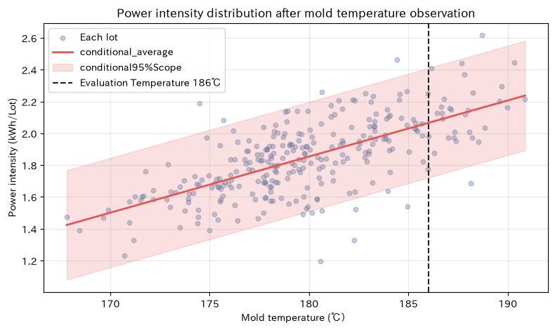
0	If you don't know the temperature	1.8466	0.2370
1	temperature=186.0℃If you learn about it	2.0652	0.1754

png

Reading the results

When the temperature is above average, the conditional average power also increases, and the standard deviation after knowing the temperature becomes smaller than the unconditional standard deviation. This allows you to create temperature-corrected monitoring zones. However, the range is a conditional distribution on the model and is not a confidence interval for average estimates. If there is extrapolation, product mixing, temperature dependence of dispersion, or equipment degradation, the premises of the formula are compromised.

No.069: Gaussian Process

Meaning in Practice

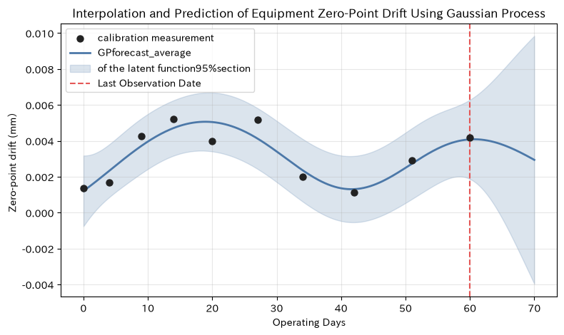
Zero-point drift in equipment changes smoothly over time, but calibration measurements are not continuous. The Gaussian process interpolates drift curves from a few measurement points, allowing for wider uncertainty in regions with fewer data. It is suitable for determining the timing of calibration and additional measurement points.

Approach to Analysis and Modeling

A Gaussian process is a probability distribution for function $f(t)$ ,

f(t)\sim\mathcal{GP}(m(t),k(t,t'))

That’s what I write. Here, the average function is 0, and the kernel is RBF.

k(t,t')=\sigma_f^2\exp\left(-\frac{(t-t')^2}{2\ell^2}\right)

and add the observed noise dispersion $\sigma_n^2$ . Predicted mean and variance are obtained from the conditionally normal distribution of the kernel matrix. $\ell$ represents the smoothness of change.

Check with Python

gp_rng = np.random.default_rng(SEED + 69)
t_obs = np.array([0, 4, 9, 14, 20, 27, 34, 42, 51, 60], dtype=float)
true_drift = lambda t: 0.004 * np.sin(t / 10) + 0.00012 * t
y_obs = true_drift(t_obs) + gp_rng.normal(0, 0.0012, len(t_obs))
t_pred = np.linspace(0, 70, 281)

length_scale = 13.0
signal_sd = 0.006
noise_sd = 0.0012

def rbf_kernel(a, b, length_scale, signal_sd):
    sq_distance = (np.asarray(a)[:, None] - np.asarray(b)[None, :]) ** 2
    return signal_sd**2 * np.exp(-0.5 * sq_distance / length_scale**2)

k_oo = rbf_kernel(t_obs, t_obs, length_scale, signal_sd) + noise_sd**2 * np.eye(len(t_obs))
k_po = rbf_kernel(t_pred, t_obs, length_scale, signal_sd)
k_pp = rbf_kernel(t_pred, t_pred, length_scale, signal_sd)
alpha = np.linalg.solve(k_oo, y_obs)
gp_mean = k_po @ alpha
v = np.linalg.solve(k_oo, k_po.T)
gp_cov = k_pp - k_po @ v
gp_sd = np.sqrt(np.clip(np.diag(gp_cov), 0, None))

gp_summary = pd.DataFrame({
    "Location": ["Last Observation Date", "10Ahead of the day"],
    "days": [60, 70],
    "forecast_average_mm": [np.interp(60, t_pred, gp_mean), np.interp(70, t_pred, gp_mean)],
    "predicted_standard_deviation_mm": [np.interp(60, t_pred, gp_sd), np.interp(70, t_pred, gp_sd)],
})
display(gp_summary.round(5))

plt.scatter(t_obs, y_obs, color="#222222", s=42, zorder=3, label="calibration measurement")
plt.plot(t_pred, gp_mean, color="#4C78A8", linewidth=2, label="GPforecast_average")
plt.fill_between(t_pred, gp_mean - 1.96 * gp_sd, gp_mean + 1.96 * gp_sd,
                 color="#4C78A8", alpha=0.2, label="of the latent function95%section")
plt.axvline(t_obs.max(), color="#E45756", linestyle="--", label="Last Observation Date")
plt.title("Interpolation and Prediction of Equipment Zero-Point Drift Using Gaussian Process")
plt.xlabel("Operating Days")
plt.ylabel("Zero-point drift (mm）")
plt.grid(alpha=0.3)
plt.legend()
plt.tight_layout()
plt.show()

	Location	days	forecast_average_mm	predicted_standard_deviation_mm
0	Last Observation Date	60	0.0041	0.0011
1	10Ahead of the day	70	0.0029	0.0035

png

Reading the results

Near the observation point, the section is narrow, but after the last observation date, it gradually expands. Not only can you predict points, but you can also use positions with increasing uncertainty as candidates for additional calibration. This time, for explanation, I fixed hyperparameters. In actual operation, estimation based on peripheral likelihood, changes due to equipment shutdowns or replacements, seasonality, and time-series verification are necessary without mixing data from the prediction point into training.

No.070: Copula

Meaning in Practice

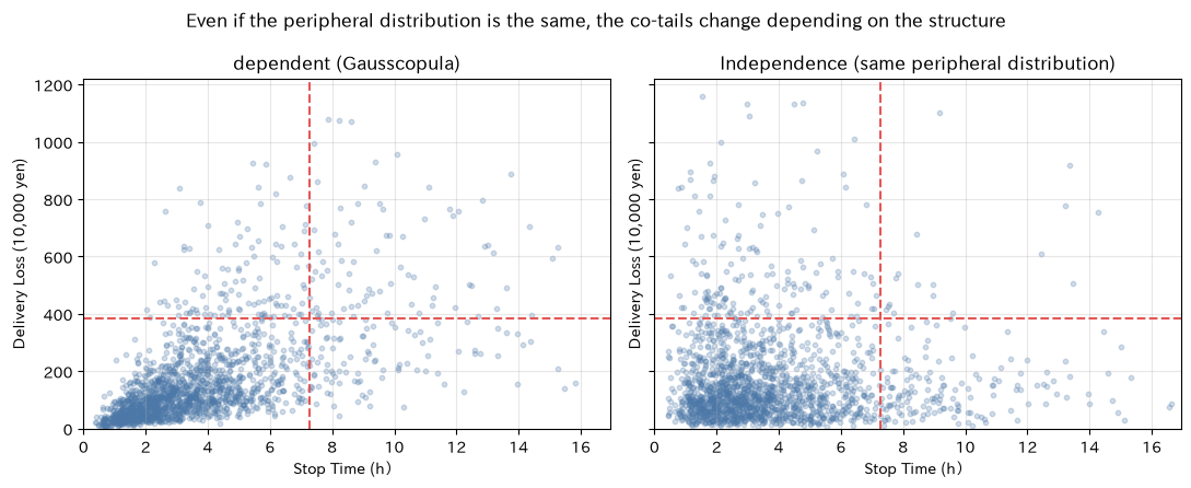
Both equipment downtime and delivery loss amounts tend to be large on the same day, both with long taillines. Copula separates the peripheral distribution and dependent structure of each indicator, and can be used for stress tests where the distribution pattern adjusts the intensity of simultaneous deterioration while keeping the distribution pattern matched to actual performance.

Approach to Analysis and Modeling

According to Sklar’s theorem, a simultaneous distribution with a continuous peripheral distribution $F_X,F_Y$ is

F_{X,Y}(x,y)=C(F_X(x),F_Y(y))

It can be expressed as such. $C$ is Copula. This time, we will use Gausscopular to map the bivariate normal random number $(Z_1,Z_2)$ with correlation $\rho$ into a uniform distribution using $U_i=\Phi(Z_i)$ and convert it to a long peripheral distribution at the right base. The comparison targets independent models with the same peripheral distribution.

Check with Python

copula_rng = np.random.default_rng(SEED + 70)
n_scenarios = 50_000
rho = 0.72
z_dep = copula_rng.multivariate_normal([0, 0], [[1, rho], [rho, 1]], size=n_scenarios)
z_ind = copula_rng.normal(size=(n_scenarios, 2))

# Log-normal transformation equivalent to passing Phi(Z) through the inverse function of the peripheral distribution
downtime_dep = np.exp(1.15 + 0.65 * z_dep[:, 0])
loss_dep = np.exp(4.80 + 0.90 * z_dep[:, 1])  # ten_thousand_yen
downtime_ind = np.exp(1.15 + 0.65 * z_ind[:, 0])
loss_ind = np.exp(4.80 + 0.90 * z_ind[:, 1])

downtime_q90 = np.quantile(downtime_dep, 0.90)
loss_q90 = np.quantile(loss_dep, 0.90)
joint_tail_dep = np.mean((downtime_dep > downtime_q90) & (loss_dep > loss_q90))
joint_tail_ind = np.mean((downtime_ind > downtime_q90) & (loss_ind > loss_q90))

copula_summary = pd.DataFrame({
    "Model": ["Gausscopular (dependent)", "Independence"],
    "median_stopping_time_h": [np.median(downtime_dep), np.median(downtime_ind)],
    "median_loss_ten_thousand_yen": [np.median(loss_dep), np.median(loss_ind)],
    "Both are each90%Probability of Surpassing Points": [joint_tail_dep, joint_tail_ind],
    "50,000Simultaneous exceedances in episodes": [joint_tail_dep * n_scenarios, joint_tail_ind * n_scenarios],
})
display(copula_summary.round(4))
print(f"90%point: Stop time {downtime_q90:.2f}Time, loss {loss_q90:.1f}ten_thousand_yen")
print(f"Simultaneous tail probability ratio: {joint_tail_dep / joint_tail_ind:.2f}double")

sample_idx = copula_rng.choice(n_scenarios, 1800, replace=False)
fig, axes = plt.subplots(1, 2, figsize=(11, 4.5), sharex=True, sharey=True)
for ax, dx, ly, title in [
    (axes[0], downtime_dep, loss_dep, "dependent (Gausscopula)"),
    (axes[1], downtime_ind, loss_ind, "Independence (same peripheral distribution)"),
]:
    ax.scatter(dx[sample_idx], ly[sample_idx], s=10, alpha=0.25, color="#4C78A8")
    ax.axvline(downtime_q90, color="#E45756", linestyle="--")
    ax.axhline(loss_q90, color="#E45756", linestyle="--")
    ax.set_title(title)
    ax.set_xlabel("Stop Time (h）")
    ax.set_ylabel("Delivery Loss (10,000 yen)")
    ax.set_xlim(0, np.quantile(downtime_dep, 0.995))
    ax.set_ylim(0, np.quantile(loss_dep, 0.995))
    ax.grid(alpha=0.3)
fig.suptitle("Even if the peripheral distribution is the same, the co-tails change depending on the structure")
plt.tight_layout()
plt.show()

	Model	median_stopping_time_h	median_loss_ten_thousand_yen	Both are each90%Probability of Surpassing Points	50,000Simultaneous exceedances in episodes
0	Gausscopular (dependent)	3.1421	121.1719	0.0487	2,435.0000
1	Independence	3.1645	122.0452	0.0092	460.0000

90% point: Downtime 7.27 hours, loss of 3,846,000 yen
Simultaneous tail probability ratio: 5.29x

png

Reading the results

The median stoppage time and loss amount for both models are almost the same, but the probability of both exceeding 90% is higher in the dependent model. It is clear that even if only the peripheral distribution is individually adjusted, simultaneous risk cannot be reproduced. Note that Gausscopular may underestimate dependence on extreme hems. For BCP applications, comparisons with t-copula and others, definitions of extreme events, parameter estimation errors, and stress scenarios are examined.

Practical Implications Seen Through Target Exercise

aloneKPIand combinationsKPIAssign roles
Peripheral distribution is concise in management reports, but simultaneous distribution is necessary for composite quality and simultaneous shutdowns.
Update probabilities with observational information
Once you know the temperature range and product, use a conditional distribution instead of the overall probability. The sample size by condition is also listed.
Do not leave the assumption of independence for convenience
In the Monte Carlo plan, accumulating risks and ignoring dependence leads to simultaneous tail errors.
Distinguishing Covariance and Correlation
If you calculate the variance of synthetic loss per unit, use covariance; if you compare relationships across units, use correlation.
Distinguishing between the model’s usual area and quality standards
The multivariate normal outside the ellipse is statistically rare and not a defective judgment itself.
Adding uncertainty to forecasts
Conditional normal distributions and Gaussian processes can pass not only averages but also forecast breadth to decision-making.
Examining peripheral distribution and dependency structure separately
In Copula, we evaluate the distribution fit of each KPI and the fit of the concurrent structure.

What is necessary for practical implementation

1. Align the analysis unit and time

We unify the particle size for lots, individuals, and equipment seconds, and connect material input, condition setting, inspection, stop, and shipment with trackable keys. It also manages sensor clock misalignment and the aggregation window.

2. Manage the definitions of KPIs, standards, and missing items

Records measuring instruments, units, upper and lower standard limits, rounding, re-measurement, supplementation of missing measurements, and equipment replacement. Do not mix probabilities before and after the standard change as the same population.

3. Confirm stratification and time series structure

The distribution may vary depending on the product, equipment, molds, materials, and work zone. In addition to random splitting, we conduct verification and drift monitoring using future periods.

4. Prepare premise assessments and alternative models

Check scatter plots, outliers, normality, multifrequency, nonlinearity, and autocorrelation. If the assumptions do not match, compare robust covariance, mixed distribution, tree model, time series model, and alternative copula.

5. Design the decision rules based on losses

Statistically unusual and business-critical are not the same. Defining missed detections, false alarms, stoppages, additional inspections, and loss of warranty fees, and agreeing on thresholds and response flows.

6. Start with small-scale parallel operations

Instead of immediately replacing existing judgments, they display them in parallel with specific equipment, reducing who checks when, and what to do into standard work. Assign responsible persons for relearning, reproofreading, and audit logs.

Conclusion

From No.061 to No.070, we examined the two-variable probability table, matrices, normal distributions, functional distributions, and copulas as a consistent topic in manufacturing.

A simultaneous distribution represents a combinatorial distribution, a peripheral distribution represents a single one, and a conditional distribution represents the probability after information acquisition
If it is independent, the coincidence probabilities are multiplied, but having only a correlation of 0 generally does not qualify as independence
The covariance matrix represents covariation in the unit size, while the correlation matrix represents a standardized linear relationship
The multivariate normal distribution is an elliptical normal region, while the conditional normal distribution can be used for post-observation updates
Gaussian processes deal with function prediction and uncertainty, while copulas deal with the separation of peripheral distributions and dependent structures

What matters in practice is not elaborate model names, but designing analytical units, conditions, assumptions, uncertainties, and response actions in sequence. First, visualize the simultaneous distribution from two to three key KPIs and start by cross-referencing them with on-site causal hypotheses.

Consultations for Corporations

At Suri Kobo, we support everything from problem organization to PoC, implementation, and on-site training for data analysis, statistical modeling, anomaly detection, and risk simulation for manufacturing industries.

Multivariable monitoring design of quality KPIs and equipment sensors
PoC for conditional forecasting and time series drift detection
Simultaneous risk simulation of stoppages, delivery dates, and inventories
Python and Statistics Training Using In-House Data
Support for integrating analysis results into on-site standards and decision-making processes

📩 Contact Us: surikobo.co.jp/contact
Please feel free to consult us first.

Reading Multiple KPIs Simultaneously—Multivariate Probabilities of Manufacturing Quality, Equipment Load, and Delivery Risks

Reading Multiple KPIs Simultaneously—Multivariate Probabilities of Manufacturing Quality, Equipment Load, and Delivery Risks

Overview

Introduction: Practical Challenges in Manufacturing Covered in This Article

Common situations on site

Why is this issue so difficult to judge?

Overview of Exercise covered this time

Preparing the Python environment

Creation of Fictional Data

No.061: Simultaneous Distribution

Meaning in Practice

Approach to Analysis and Modeling

Check with Python

Reading the results

No.062: Peripheral Distribution

Meaning in Practice

Approach to Analysis and Modeling

Check with Python

Reading the results

No.063: Conditional Distribution

Meaning in Practice

Approach to Analysis and Modeling

Check with Python

Reading the results

No.064: Independence

Meaning in Practice

Approach to Analysis and Modeling

Check with Python

Reading the results

No.065: Covariance Matrix

Meaning in Practice

Approach to Analysis and Modeling

Check with Python

Reading the results

No.066: Correlation Matrix

Meaning in Practice

Approach to Analysis and Modeling

Check with Python

Reading the results

No.067: Multivariate Normal Distribution

Meaning in Practice

Approach to Analysis and Modeling

Check with Python

Reading the results

No.068: Conditional Normal Distribution

Meaning in Practice

Approach to Analysis and Modeling

Check with Python

Reading the results

No.069: Gaussian Process

Meaning in Practice

Approach to Analysis and Modeling

Check with Python

Reading the results

No.070: Copula

Meaning in Practice

Approach to Analysis and Modeling

Check with Python

Reading the results

Practical Implications Seen Through Target Exercise

What is necessary for practical implementation

1. Align the analysis unit and time

2. Manage the definitions of KPIs, standards, and missing items

3. Confirm stratification and time series structure

4. Prepare premise assessments and alternative models

5. Design the decision rules based on losses

6. Start with small-scale parallel operations

Conclusion

Consultations for Corporations

Related Posts

Don't End Process Changes with 'Feels Like It's Working'—Judging Quality Investment with Statistical Reasoning

Learning Manufacturing Statistical Estimation with Python | From Sampling Inspections to EM Algorithms

Turning sample size into a basis for quality judgment—10 exercises on the extreme limit theorem for manufacturing KPIs

How to Estimate Failure, Quality, and Maintenance Time—10 Continuous Distribution Options Used in Manufacturing

Predicting Manufacturing Defects and Equipment Downtime Using Discrete Distribution | 10 Practical Tips for Python