How many defects and stoppages occur? — Developing inspection and maintenance plans at manufacturing sites based on discrete distribution

Overview

On the manufacturing floor, Events Counted by Integers are handled daily, including the presence or absence of defects, the number of defects found in a certain number of inspections, the interval between the next abnormality, and the number of equipment alarms. In this article, using a fictional electronic components factory as a subject, we connect ten discrete distributions—from Bernoulli distributions to the Poisson process—to decisions regarding quality assurance, incoming inspection, and maintenance personnel assignment.

The subject is the No.041〜No.050 of ‘100 Exercises on Probability and Statistical Theory.’ Not only does it use formulas, but we also verify the differences in premise in Python: “Should we fix the number of trials?”, “Should we wait until the number of occurrences?”, or “Should we extract without returning from the population?”

[!NOTE] This material is a notebook previously used by Surikoubo (or personally by the representative, Kazuyama), and has been reconstructed, edited, and published with the company’s permission.
All data listed is fictional and has no relation whatsoever to real companies, factories, or figures.

Introduction: Practical Challenges in Manufacturing Covered in This Article

This time, the subject is a fictional factory that produces 400 sensor boards per day. The quality assurance and equipment maintenance departments must answer the following questions with limited staff.

• How to express the probability of a single product defecting in the smallest unit
• How to estimate the number of defects per day or the probability of “days when 5 or more defects occur”
• How many will be inspected before the next defect or the fifth defect?
• For sampling from finite lots, is it acceptable to use the binomial distribution as is?
• How to evaluate the number of facility alarms and the probability of exceeding response capacity within the time limit
• How to allocate personnel, parts, and analysis man-hours by defect cause
• When can the binomial distribution of rare defects be approximated using the Poisson distribution?
• How should we consider conservation plans, including not only the number of cases but also the time of occurrence?

Discrete distribution quantifies excess probability and wait times by selecting assumptions that match the phenomena alone, which cannot be seen by the average number of cases.

Common situations on site

On site, average values such as “defect rate 1.2%” and “an average of 0.65 alarms per hour” are shared. However, in daily operations, the following misunderstandings occur.

1. Only looking at the average number of defects is not securing the necessary inspectors on the upward day.
2. A binomial model that returns sampling to the population is used to approximate the sample, without considering finite lot correction.
3. Treats ‘up to the next one’ and ‘until five occurrences’ are treated with the same distribution.
4. The number of cases by cause is calculated as an independent binomial distribution, and the total number of cases does not match.
5. The daily number of cases only appears to be a Poisson distribution, but it is judged that temporal independence and a certain incidence rate are established.

Rather than memorizing distribution names, it is important to decide what to fix and what to use as random variables.

Why is this issue so difficult to judge?

First, even similar formulas have different sample designs. A binomial distribution is a model that repeats a fixed number of independent trials with a fixed probability, while the hypergeometric distribution extracts from a finite population without returning it. The higher the extraction rate, the harder the difference between the two cannot be ignored.

Second, the random variables vary depending on the KPIs you want to manage. The “number of defects out of 400” is a binomial distribution, the number of tests up to the first defect is a geometric distribution, and the number of tests up to the fifth is a negative binomial distribution.

Third, there are additional assumptions about the Poisson distribution and Poisson process. Even if the number of incidents within a certain period is a Poisson distribution, if there are seasonality, equipment conditions, or the effects of previous stoppages, the assumption of a constant incidence rate and independent increment process is rejected. In practice, it is necessary to check not only the suitability but also the time-of-day trends and continuous occurrences.

Overview of Exercise covered this time

No.	Theme	Questions in the Manufacturing Industry
041	Bernoulli distribution	How to Indicate Good or Defective Individual Products
042	binomial distribution	When inspecting the fixed quantity, how many defects are there
043	geometric distribution	How many defects should be inspected up to the first time?
044	Negative binomial distribution	How many tests are needed until the fifth defect?
045	hypergeometric distribution	What is the probability of accepting a limited lot lot?
046	Poisson distribution	Several facility alarms for certain periods
047	multiplenic distribution	How to allocate the total number of defects by cause
048	Category distribution	How to probabilistically represent the cause of a single defect
049	Poisson limit theorem	Can a binomial distribution of rare defects be approximated?
050	Poisson process	How to handle the number of alarms and their activation times

No.041 is the smallest unit for individual item determination, and the process is expanded sequentially to fixed count, waiting time, non-restorative extraction, multiple classification, rare events, and time axis.

Preparing the Python environment

Generate fictional data and simulations with NumPy, create tables with pandas, calculate theoretical probabilities with SciPy, and visualize them with matplotlib. Regardless of external data, fix the random seed so that it can be rerun and achieve the same result.

import sys
import platform

import matplotlib
import matplotlib.pyplot as plt
import numpy as np
import pandas as pd
import scipy
from scipy.special import comb
from scipy.stats import binom, geom, hypergeom, poisson
import japanize_matplotlib  # noqa: F401 Japanese font settings
from IPython.display import display

SEED = 20260711
rng = np.random.default_rng(SEED)

pd.set_option("display.max_columns", 20)
pd.set_option("display.float_format", lambda x: f"{x:,.4f}")
plt.rcParams["figure.figsize"] = (8, 4.5)
plt.rcParams["axes.unicode_minus"] = False

print(f"Python: {sys.version.split()[0]}")
print(f"OS: {platform.system()} {platform.release()}")
print(f"NumPy: {np.__version__}")
print(f"pandas: {pd.__version__}")
print(f"SciPy: {scipy.__version__}")
print(f"matplotlib: {matplotlib.__version__}")
print(f"random number seed: {SEED}")

Python: 3.13.1
OS: Darwin 25.3.0
NumPy: 2.5.1
pandas: 3.0.3
SciPy: 1.18.0
matplotlib: 3.11.0
Random number seed: 20260711

Creation of Fictional Data

For 60 operating days, it generates 400 defects per day, equipment alarms within 8 hours, and the number of defect cases by cause. The reference values on the model are as follows:

• Probability of defective items: $p=0.012$ (1.2%)
• Equipment alarm occurrence rate: $\lambda=0.65$ per hour
• Defect cause composition: Solder 45%, parts 25%, mounting misalignment 20%, others 10%
• Each day’s trial is assumed to be independent under the same conditions

The final assumption is simplification in the teaching materials. In practical data, we first check whether probabilities have changed due to equipment units, varieties, material lots, working hours, recipe changes, or elapsed time after maintenance.

n_days = 60
units_per_day = 400
defect_probability = 0.012
hours_per_day = 8
alarm_rate_per_hour = 0.65
cause_names = np.array(["solder", "Parts", "Implementation Misalignment", "Other"])
cause_probabilities = np.array([0.45, 0.25, 0.20, 0.10])

daily_defects = rng.binomial(units_per_day, defect_probability, size=n_days)
daily_alarms = rng.poisson(hours_per_day * alarm_rate_per_hour, size=n_days)
daily_causes = np.vstack([
    rng.multinomial(count, cause_probabilities) for count in daily_defects
])

df = pd.DataFrame({
    "Operating Days": pd.date_range("2026-04-01", periods=n_days, freq="D"),
    "production_volume": units_per_day,
    "number_of_defects": daily_defects,
    "non_performing_rate": daily_defects / units_per_day,
    "Number of facility alarms": daily_alarms,
})
for i, cause in enumerate(cause_names):
    df[f"cause_{cause}"] = daily_causes[:, i]

display(df.head(10))
summary = pd.DataFrame({
    "indicator": ["Daily defective count", "daily defect rate", "Daily Number of Equipment Alarms"],
    "Average performance": [df["number_of_defects"].mean(), df["non_performing_rate"].mean(), df["Number of facility alarms"].mean()],
    "Model Expectations": [units_per_day * defect_probability, defect_probability,
                   hours_per_day * alarm_rate_per_hour],
})
display(summary.round(4))
print(f"Number of missing items: {int(df.isna().sum().sum())} / Total number of cells: {df.size:,}")

	Operating Days	production_volume	number_of_defects	non_performing_rate	Number of facility alarms	cause_solder	cause_Parts	cause_Implementation Misalignment	cause_Other
0	2026-04-01	400	3	0.0075	5	2	0	1	0
1	2026-04-02	400	8	0.0200	7	5	0	2	1
2	2026-04-03	400	5	0.0125	3	1	2	0	2
3	2026-04-04	400	6	0.0150	5	4	0	0	2
4	2026-04-05	400	7	0.0175	5	1	3	3	0
5	2026-04-06	400	3	0.0075	9	2	1	0	0
6	2026-04-07	400	2	0.0050	3	0	2	0	0
7	2026-04-08	400	8	0.0200	2	3	2	3	0
8	2026-04-09	400	5	0.0125	7	0	2	3	0
9	2026-04-10	400	4	0.0100	9	1	0	3	0

	indicator	Average performance	Model Expectations
0	Daily defective count	4.8333	4.8000
1	daily defect rate	0.0121	0.0120
2	Daily Number of Equipment Alarms	5.1167	5.2000

Number of Missing Cells: 0 / Total Cells: 540

---

No.041: Bernoulli Distribution

Meaning in Practice

The Bernoulli distribution expresses a single test result as a binary value: ‘Defective = 1, Good Product = 0.’ This is the minimum model for binary KPIs, such as pass/fail judgments for individual items, equipment shutdown status, and on-time delivery success.

Approach to Analysis and Modeling

$X\in\{0,1\}$, if the defect probability is $p$, then the probability mass function, expected value, and variance are

$$P(X=x)=p^x(1-p)^{1-x},\qquad E[X]=p,\qquad V[X]=p(1-p)$$

That’s right. The sample mean of 0/1 data is the defect rate as is. However, if the $p$ differs by product, the assumption that all data is considered the same Bernoulli trial is compromised.

Check with Python

bernoulli_table = pd.DataFrame({
    "determination_x": [0, 1],
    "Meaning": ["good product", "bad"],
    "probability_p(X=x)": [1 - defect_probability, defect_probability],
})
display(bernoulli_table)
print(f"theoretical expected value E[X] = p: {defect_probability:.4f}")
print(f"theoretical dispersion V[X] = p(1-p): {defect_probability * (1-defect_probability):.6f}")

plt.bar(bernoulli_table["Meaning"], bernoulli_table["probability_p(X=x)"], color=["#4C78A8", "#E45756"])
plt.title("Bernoulli distribution in individual inspection")
plt.xlabel("Inspection Judgment")
plt.ylabel("probability")
plt.grid(axis="y", alpha=0.3)
plt.tight_layout()
plt.show()

	determination_x	Meaning	probability_P(X=x)
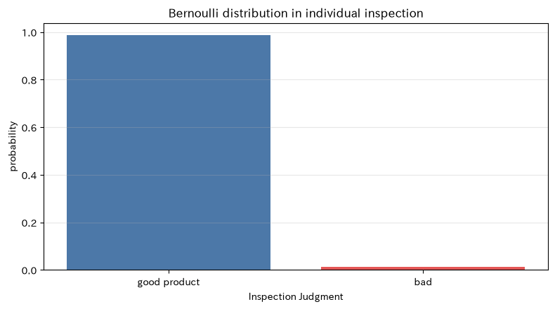
0	0	good product	0.9880
1	1	bad	0.0120

Theoretical expected value E[X] = p: 0.0120
Theoretical variance V[X] = p(1 - p): 0.011856

Reading the results

A single inspection only observes either good or defective products, but by accumulating many 0/1s and averaging them, the defect rate can be estimated. The defect probability of 1.2% is not a value that predicts defects in individual products, but rather a long-term ratio when many are produced under the same conditions. Before mixing equipment, varieties, and periods, it is necessary to define management units that can be considered the same $p$.

---

No.042: Binomial Distribution

Meaning in Practice

The binomial distribution represents how many defects occur within a fixed number of production and inspection numbers. Not only the average number of defects, but also the probability of upside failures requiring re-inspections or support staff can be calculated.

Approach to Analysis and Modeling

If we run $n$ independent Bernoulli trials and set the number of defects to $X$,

$$X\sim\operatorname{Bin}(n,p),\quad P(X=k)=\binom{n}{k}p^k(1-p)^{n-k}$$

So, $E[X]=np$, $V[X]=np(1-p)$. Assuming 400 units per day and $p=0.012$, the probability of 5 or more defects occurring is calculated.

Check with Python

k = np.arange(0, 16)
binom_pmf = binom.pmf(k, units_per_day, defect_probability)
tail_probability = binom.sf(4, units_per_day, defect_probability)

binom_table = pd.DataFrame({"number_of_defects_k": k, "probability": binom_pmf})
display(binom_table.round(5))
print(f"Expected defects np: {units_per_day * defect_probability:.2f} units/days")
print(f"standard_deviation: {np.sqrt(units_per_day * defect_probability * (1-defect_probability)):.2f} units")
print(f"5Probability of being more than one P(X>=5): {tail_probability:.2%}")

plt.bar(k, binom_pmf, color="#4C78A8")
plt.axvline(4.5, color="#E45756", linestyle="--", label="5more than several")
plt.title("1days400Number of defects during individual production (binomial distribution)")
plt.xlabel("1Number of defective items per day")
plt.ylabel("probability")
plt.grid(axis="y", alpha=0.3)
plt.legend()
plt.tight_layout()
plt.show()

	number_of_defects_k	probability
0	0	0.0080
1	1	0.0388
2	2	0.0941
3	3	0.1516
4	4	0.1828
5	5	0.1758
6	6	0.1406
7	7	0.0961
8	8	0.0573
9	9	0.0303
10	10	0.0144
11	11	0.0062
12	12	0.0024
13	13	0.0009
14	14	0.0003
15	15	0.0001

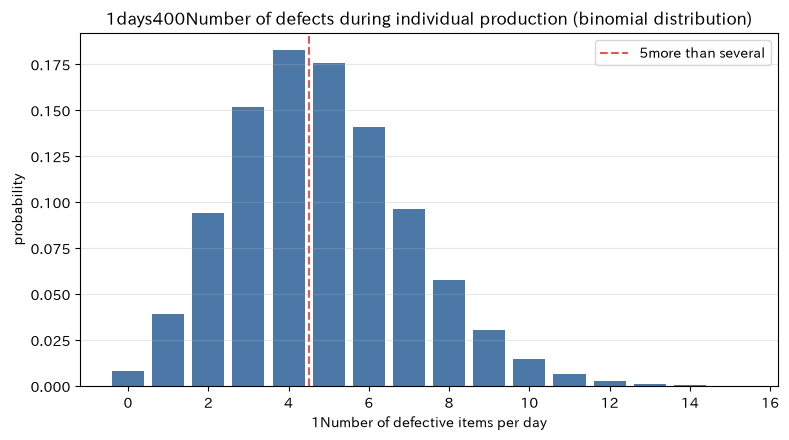
Expected defects np: 4.80 units/day
Standard Deviation: 2.18
Probability of 5 or more P(X>=5): 52.46%

Reading the results

The expected value is 4.8, but the probability of getting more than 5 is about 5. “Five is more than average, so it’s not abnormal.” The daily management warning line is set not by simple comparison with the average but by acceptable overtime frequency and loss amounts. Also, if the defect probability changes over consecutive days, a model by product type and equipment condition is needed rather than a single binomial distribution.

---

No.043: Geometric Distribution

Meaning in Practice

The geometric distribution represents how many items will be inspected before the first defect is found. This serves as an entry point for considering the estimated number of consecutive good products, the interval between patrol inspections, and the inspection load until abnormalities are detected.

Approach to Analysis and Modeling

If $T$ is the number of tests including the initial defect,

$$P(T=t)=(1-p)^{t-1}p,\quad t=1,2,\ldots$$

So, it’s $E[T]=1/p$. The geometric distribution has a memoryless nature: “No matter how many good products have been produced so far, the probability of defects for the next one remains $p$.” In sites where process degradation progresses, this assumption is carefully verified.

Check with Python

t = np.arange(1, 401)
geom_pmf = geom.pmf(t, defect_probability)
q50, q90, q95 = geom.ppf([0.50, 0.90, 0.95], defect_probability).astype(int)

geom_summary = pd.DataFrame({
    "indicator": ["average", "median", "90%quantile", "95%quantile"],
    "Number of Tests": [1 / defect_probability, q50, q90, q95],
})
display(geom_summary.round(1))

plt.plot(t, geom.cdf(t, defect_probability), color="#4C78A8", label="cumulative probability")
plt.axhline(0.90, color="#E45756", linestyle="--", label="90%")
plt.axvline(q90, color="#E45756", linestyle=":", label=f"{q90}units")
plt.title("Number of tests until the first defect is found")
plt.xlabel("Number of tests including initial defects")
plt.ylabel("cumulative probability P(T <= t)")
plt.grid(alpha=0.3)
plt.legend()
plt.tight_layout()
plt.show()

	indicator	Number of Tests
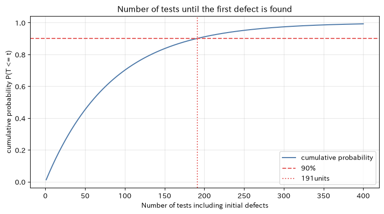
0	average	83.3000
1	median	58.0000
2	90%quantile	191.0000
3	95%quantile	249.0000

Reading the results

The average is about 83, but the distribution is long to the right, and the number of tests with a 90% chance of finding the first defect is significantly higher than average. Designing patrol inspections based solely on average intervals can overestimate the probability of detection. The inspection interval is determined based on the service level of “what percentage of probability we want to detect abnormalities.”

---

No.044: Negative Binomial Distribution

Meaning in Practice

The negative binomial distribution represents the number of tests required before a specified number of defects are found. For example, the inspection man-hours and period until five defective products are secured for cause analysis can be estimated.

Approach to Analysis and Modeling

If $T_r$ is the number of tests including $r$ defects,

$$P(T_r=t)=\binom{t-1}{r-1}p^r(1-p)^{t-r},\quad t=r,r+1,\ldots$$

So, $E[T_r]=r/p$, $V[T_r]=r(1-p)/p^2$. SciPy nbinom returns “up to $r$ good products,” so when converting to the total number of inspections, note that $r$ is added.

Check with Python

r = 5
total_inspections = np.arange(r, 1201)
good_before_rth_defect = total_inspections - r
nb_pmf = scipy.stats.nbinom.pmf(good_before_rth_defect, r, defect_probability)
nb_quantiles = scipy.stats.nbinom.ppf([0.50, 0.90, 0.95], r, defect_probability) + r

nb_summary = pd.DataFrame({
    "indicator": ["average", "median", "90%quantile", "95%quantile"],
    "Total number of tests": [r / defect_probability, *nb_quantiles],
})
display(nb_summary.round(1))

plt.plot(total_inspections, scipy.stats.nbinom.cdf(good_before_rth_defect, r, defect_probability),
         color="#59A14F")
plt.axhline(0.90, color="#E45756", linestyle="--", label="90%")
plt.axvline(nb_quantiles[1], color="#E45756", linestyle=":", label=f"{nb_quantiles[1]:.0f}units")
plt.title("5Total number of inspections until defective items are secured")
plt.xlabel("Total number of tests")
plt.ylabel("cumulative probability")
plt.grid(alpha=0.3)
plt.legend()
plt.tight_layout()
plt.show()

	indicator	Total number of tests
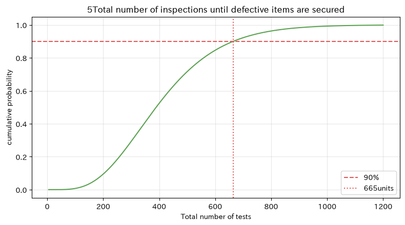
0	average	416.7000
1	median	389.0000
2	90%quantile	665.0000
3	95%quantile	761.0000

Reading the results

The average number of inspections up to 5 is about 417, but even greater testing capacity is needed to secure 90% accuracy. If you only promise the start date for cause analysis based on the average, delays are likely to occur, so plan based on the quantile. In processes where defects are concentrated, the assumption of independence and constant probability is broken, and the actual variance may be larger than in this model.

---

No.045: Hypergeometric Distribution

Meaning in Practice

The metageometric distribution is suitable for acceptance inspections that extract without returning of products from finite lots. Assuming the number of defects in a lot is known, this represents how many defects will be found in the sample.

Approach to Analysis and Modeling

For total lot $N$, defective count $D$, extraction number $n$, and detected defects $X$,

$$P(X=k)=\frac{\binom{D}{k}\binom{N-D}{n-k}}{\binom{N}{n}}$$

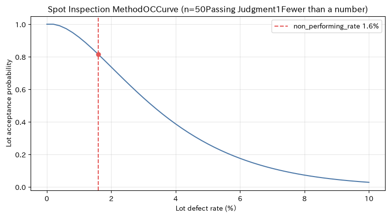
That’s right. Here, we use $N=500$, $D=8$, $n=50$, and calculate the acceptance probability of the rule accepting one or fewer defects. This is the probability of accepting lots of a specific quality, and the quality of the extraction method is evaluated by the OC curve for multiple $D$.

Check with Python

N, D, sample_n, acceptance_c = 500, 8, 50, 1
x_h = np.arange(0, min(D, sample_n) + 1)
h_pmf = hypergeom.pmf(x_h, N, D, sample_n)
acceptance_probability = hypergeom.cdf(acceptance_c, N, D, sample_n)

display(pd.DataFrame({"Number of defective samples": x_h, "probability": h_pmf}).round(6))
print(f"bad1Probability of accepting fewer than one: {acceptance_probability:.2%}")

defect_counts = np.arange(0, 51)
oc_curve = hypergeom.cdf(acceptance_c, N, defect_counts, sample_n)
plt.plot(defect_counts / N * 100, oc_curve, color="#4C78A8")
plt.axvline(D / N * 100, color="#E45756", linestyle="--", label=f"non_performing_rate {D/N:.1%}")
plt.scatter([D / N * 100], [acceptance_probability], color="#E45756", zorder=3)
plt.title("Spot Inspection MethodOCCurve (n=50Passing Judgment1Fewer than a number)")
plt.xlabel("Lot defect rate (%）")
plt.ylabel("Lot acceptance probability")
plt.grid(alpha=0.3)
plt.legend()
plt.tight_layout()
plt.show()

	Number of defective samples	probability
0	0	0.4278
1	1	0.3862
2	2	0.1492
3	3	0.0322
4	4	0.0042
5	5	0.0003
6	6	0.0000
7	7	0.0000
8	8	0.0000

Probability of accepting one or fewer defects: 81.40%

Reading the results

Even if a lot contains eight defects, there is a possibility that the sampling result will be one or fewer, making it acceptable. Spot checks are not guaranteed to be all-in-one; rather, it is a distribution of producer risk for mistakenly rejecting good lots and consumer risk for accepting bad lots. We design not only acceptable quality levels but also $n$ and pass quantity by combining losses from major defects and inspection costs.

---

No.046: Poisson Distribution

Meaning in Practice

The Poisson distribution represents a relatively rare number of events occurring over a fixed time, area, and duration. It can be used for facility alarms, foreign object defects, inquiries, and minor stoppage capability planning.

Approach to Analysis and Modeling

If the average number of occurrences during the period is $\lambda$,

$$P(X=k)=e^{-\lambda}\frac{\lambda^k}{k!},\qquad E[X]=V[X]=\lambda$$

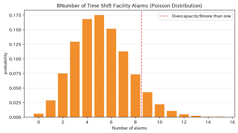
That’s right. In this example, there are $\lambda=0.65\times8=5.2$ cases per 8 hours. A characteristic is that the average and variance are equal, but if the actual variance is large, fluctuations in incidence rates or concentrated occurrence are suspected.

Check with Python

lambda_day = alarm_rate_per_hour * hours_per_day
alarm_k = np.arange(0, 16)
alarm_pmf = poisson.pmf(alarm_k, lambda_day)
over_capacity_probability = poisson.sf(8, lambda_day)

poisson_check = pd.DataFrame({
    "item": ["theoretical mean", "theoretical dispersion", "Average performance", "Diversification of Performance(ddof=1)", "9Probability of more than one"],
    "value": [lambda_day, lambda_day, df["Number of facility alarms"].mean(),
          df["Number of facility alarms"].var(ddof=1), over_capacity_probability],
})
display(poisson_check.round(4))

plt.bar(alarm_k, alarm_pmf, color="#F28E2B")
plt.axvline(8.5, color="#E45756", linestyle="--", label="Overcapacity:9more than one")
plt.title("8Number of Time Shift Facility Alarms (Poisson Distribution)")
plt.xlabel("Number of alarms")
plt.ylabel("probability")
plt.grid(axis="y", alpha=0.3)
plt.legend()
plt.tight_layout()
plt.show()

	item	value
0	theoretical mean	5.2000
1	theoretical dispersion	5.2000
2	Average performance	5.1167
3	Diversification of Performance(ddof=1)	5.0879
4	9Probability of more than one	0.0819

Reading the results

Even if an average of 5.2 shifts occur, there is a certain probability that there will be 9 or more cases on the day. If you match the capacity of maintenance personnel to the average number of cases, the number of waiting days for recovery accumulates over the number of days. On the other hand, since the actual difference between average and variance fluctuates over about 60 days, it is not immediately confirmed as model non-conformity; instead, periods, equipment stratification, and continuous occurrence confirmation are performed.

---

No.047: Multipleive Distribution

Meaning in Practice

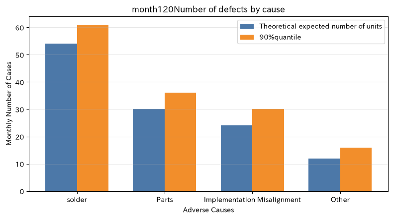
A multiple-level distribution is a model that allocates a fixed total number of cases into multiple mutually exclusive categories. We categorize the total number of defects by cause and respond to situations where analysts estimate the required amount of replacement parts.

Approach to Analysis and Modeling

If $n$ are classified into $K$ categories, the number of cases is $\mathbf{X}=(X_1,\ldots,X_K)$, and the probability is $\mathbf{p}$,

$$P(\mathbf{X}=\mathbf{x})=\frac{n!}{\prod_{j=1}^K x_j!}\prod_{j=1}^Kp_j^{x_j}, \quad \sum_jx_j=n,\quad \sum_jp_j=1$$

That’s right. $E[X_j]=np_j$ is fixed, so there is a negative covariance $\operatorname{Cov}(X_i,X_j)=-np_ip_j$ between categories because the total number of entries is fixed.

Check with Python

monthly_total = 120
n_simulations = 20_000
simulated_causes = rng.multinomial(monthly_total, cause_probabilities, size=n_simulations)

multinomial_summary = pd.DataFrame({
    "cause": cause_names,
    "Cause Probability": cause_probabilities,
    "Theoretical expected number of units": monthly_total * cause_probabilities,
    "simulation mean": simulated_causes.mean(axis=0),
    "90%quantile": np.quantile(simulated_causes, 0.90, axis=0),
})
display(multinomial_summary.round(2))
print(f"The total number of causes in each simulation{monthly_total}records: "
      f"{np.all(simulated_causes.sum(axis=1) == monthly_total)}")
print(f"Experience covariance in solder count and part count: {np.cov(simulated_causes[:, 0], simulated_causes[:, 1], ddof=0)[0,1]:.2f}")

xpos = np.arange(len(cause_names))
plt.bar(xpos - 0.18, monthly_total * cause_probabilities, width=0.36, label="Theoretical expected number of units", color="#4C78A8")
plt.bar(xpos + 0.18, np.quantile(simulated_causes, 0.90, axis=0), width=0.36,
        label="90%quantile", color="#F28E2B")
plt.xticks(xpos, cause_names)
plt.title("month120Number of defects by cause")
plt.xlabel("Adverse Causes")
plt.ylabel("Monthly Number of Cases")
plt.grid(axis="y", alpha=0.3)
plt.legend()
plt.tight_layout()
plt.show()

	cause	Cause Probability	Theoretical expected number of units	simulation mean	90%quantile
0	solder	0.4500	54.0000	53.9400	61.0000
1	Parts	0.2500	30.0000	30.0100	36.0000
2	Implementation Misalignment	0.2000	24.0000	24.0300	30.0000
3	Other	0.1000	12.0000	12.0200	16.0000

Total number of causes in each simulation is 120: True
Experience covariance between number of solder and number of parts: -13.46

Reading the results

The expected number of cases refers to the standard quantity of personnel and parts, while the 90th percentile is the candidate capacity to prepare for the upside. If each number of causes is treated as a separate independent binomial distribution, the total can exceed or fall below 120. If you are handling cause construction with a fixed total number of cases, you need to maintain the constraints of multinomial distribution and dependencies between categories.

---

No.048: Category Distribution

Meaning in Practice

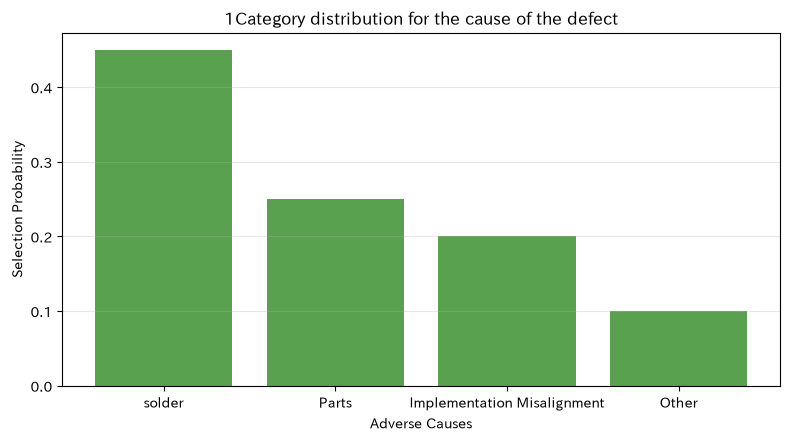
Category distribution is a model that classifies a single defect into one of multiple causes. If the multinomial distribution aggregates multiple entries, the category distribution corresponds to that one item. The output probability of the automatic cause classification model can be expressed in the same form.

Approach to Analysis and Modeling

For a one-hot vector $\mathbf{x}$ representing category $j$,

$$P(\mathbf{X}=\mathbf{x})=\prod_{j=1}^K p_j^{x_j}, \qquad x_j\in\{0,1\},\quad \sum_jx_j=1$$

That’s right. Since categories do not have numerical values, the average value of “solder = 1, parts = 2” has no practical significance. Handled with probability or one-hot expressions.

Check with Python

n_examples = 12
sampled_causes = rng.choice(cause_names, size=n_examples, p=cause_probabilities)
categorical_df = pd.DataFrame({"badID": [f"D{i:03d}" for i in range(1, n_examples + 1)],
                               "Cause category": sampled_causes})
one_hot = pd.get_dummies(categorical_df["Cause category"], dtype=int).reindex(columns=cause_names, fill_value=0)
display(pd.concat([categorical_df, one_hot], axis=1))

category_table = pd.DataFrame({"Cause category": cause_names, "probability": cause_probabilities})
plt.bar(category_table["Cause category"], category_table["probability"], color="#59A14F")
plt.title("1Category distribution for the cause of the defect")
plt.xlabel("Adverse Causes")
plt.ylabel("Selection Probability")
plt.grid(axis="y", alpha=0.3)
plt.tight_layout()
plt.show()

	badID	Cause category	solder	Parts	Implementation Misalignment	Other
0	D001	Other	0	0	0	1
1	D002	Parts	0	1	0	0
2	D003	Parts	0	1	0	0
3	D004	solder	1	0	0	0
4	D005	solder	1	0	0	0
5	D006	solder	1	0	0	0
6	D007	Implementation Misalignment	0	0	1	0
7	D008	solder	1	0	0	0
8	D009	Implementation Misalignment	0	0	1	0
9	D010	solder	1	0	0	0
10	D011	solder	1	0	0	0
11	D012	Other	0	0	0	1

Reading the results

Each row’s one-hot column must always be one 1, and this assumes that multiple causes are not classified as definite at once. In practice, since there may be complex causes or unknown causes, classification rules are defined first. Even when using AI classification probabilities, it is necessary to design thresholds that do not rely solely on maximum probability to confirm and to assign low-reliability cases to manual confirmation.

---

No.049: Poisson Limit Theorem

Meaning in Practice

The Poisson limit theorem is the basis for approximating a binomial distribution with a large number of attempts and a low success probability using a Poisson distribution that is easy to compute. It helps estimate the number of rare defects in mass production.

Approach to Analysis and Modeling

When $n\to\infty$, $p\to0$, $np\to\lambda$

$$\operatorname{Bin}(n,p)\ \Rightarrow\ \operatorname{Poisson}(\lambda)$$

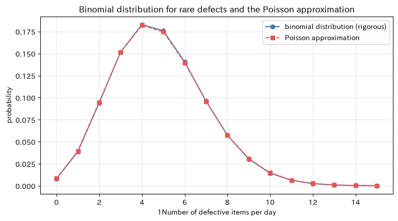
That’s how it works. Since finite $n,p$ has approximate errors, the probability mass function and the tail probability are compared in the $n=400,p=0.012,\lambda=4.8$ of this example. Even if the average $np$ is the same, if the $p$ is large, the approximation will be poor.

Check with Python

lambda_defects = units_per_day * defect_probability
compare_k = np.arange(0, 16)
exact = binom.pmf(compare_k, units_per_day, defect_probability)
approx = poisson.pmf(compare_k, lambda_defects)
comparison = pd.DataFrame({
    "number_of_defects": compare_k,
    "binomial_distribution_strict": exact,
    "Poisson approximation": approx,
    "absolute error": np.abs(exact - approx),
})
display(comparison.round(6))
print(f"Maximum absolute error within display range: {comparison['absolute error'].max():.6f}")
print(f"P(X>=10) binomial_distribution: {binom.sf(9, units_per_day, defect_probability):.4%}")
print(f"P(X>=10) Poisson approximation: {poisson.sf(9, lambda_defects):.4%}")

plt.plot(compare_k, exact, marker="o", label="binomial distribution (rigorous)", color="#4C78A8")
plt.plot(compare_k, approx, marker="s", linestyle="--", label="Poisson approximation", color="#E45756")
plt.title("Binomial distribution for rare defects and the Poisson approximation")
plt.xlabel("1Number of defective items per day")
plt.ylabel("probability")
plt.grid(alpha=0.3)
plt.legend()
plt.tight_layout()
plt.show()

	number_of_defects	binomial_distribution_strict	Poisson approximation	absolute error
0	0	0.0080	0.0082	0.0002
1	1	0.0388	0.0395	0.0007
2	2	0.0941	0.0948	0.0007
3	3	0.1516	0.1517	0.0001
4	4	0.1828	0.1820	0.0008
5	5	0.1758	0.1747	0.0011
6	6	0.1406	0.1398	0.0008
7	7	0.0961	0.0959	0.0003
8	8	0.0574	0.0575	0.0002
9	9	0.0303	0.0307	0.0003
10	10	0.0144	0.0147	0.0003
11	11	0.0062	0.0064	0.0002
12	12	0.0024	0.0026	0.0001
13	13	0.0009	0.0009	0.0001
14	14	0.0003	0.0003	0.0000
15	15	0.0001	0.0001	0.0000

Maximum absolute error in display range: 0.001093
P(X>=10) binomial distribution: 2.4368%
P(X>=10) Poisson approximation: 2.5141%

Reading the results

Under these conditions, the shape of the center part matches well, and the Poisson approximation can be used for approximations. However, when small differences in the probability of hem are directly linked to costs, such as acceptance judgments or major quality incidents, if calculusable, the exact value of the binomial distribution is used. We check not only the “large $n$” but also the conditions such as “the $p$ being sufficiently small” and “the trial is largely independent.”

---

No.050: Poisson Process

Meaning in Practice

The Poisson process deals not only with the number of incidents over a certain period but also with When equipment alarms occur. This is the foundation for considering maintenance loads by time of day, the time before the next call, and the probability of needing support staff.

Approach to Analysis and Modeling

In the homogeneous Poisson process $\{N(t)\}$ with an incidence rate of $\lambda$ cases per hour,

$$N(t)\sim\operatorname{Poisson}(\lambda t)$$

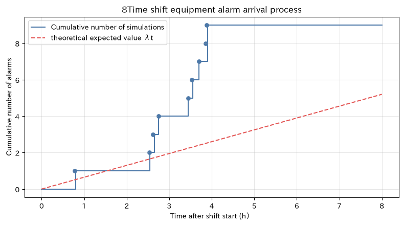
The number of cases in non-overlapping time intervals is independent. Also, the interval between arrivals $W$ follows the exponential distribution, $P(W>w)=e^{-\lambda w}$, and $E[W]=1/\lambda$. Here, we simulate the timing of one shift and compare the cumulative number of cases per hour with the theoretical expected value.

Check with Python

arrival_rng = np.random.default_rng(SEED + 50)
interarrival_times = arrival_rng.exponential(scale=1 / alarm_rate_per_hour, size=100)
arrival_times = np.cumsum(interarrival_times)
arrival_times = arrival_times[arrival_times <= hours_per_day]

time_grid = np.linspace(0, hours_per_day, 161)
cumulative_counts = np.searchsorted(arrival_times, time_grid, side="right")
process_summary = pd.DataFrame({
    "indicator": ["Number of Events in This Shift", "Theoretical expected number of units", "Average Arrival Interval(hours)",
           "2within the time limit3Probability of more than one"],
    "value": [len(arrival_times), alarm_rate_per_hour * hours_per_day, 1 / alarm_rate_per_hour,
          poisson.sf(2, alarm_rate_per_hour * 2)],
})
display(process_summary.round(4))
display(pd.DataFrame({"alarm number": np.arange(1, len(arrival_times) + 1),
                      "time_of_occurrence_h": arrival_times}).round(3))

plt.step(time_grid, cumulative_counts, where="post", label="Cumulative number of simulations", color="#4C78A8")
plt.plot(time_grid, alarm_rate_per_hour * time_grid, linestyle="--", label="theoretical expected value λt", color="#E45756")
plt.scatter(arrival_times, np.arange(1, len(arrival_times) + 1), color="#4C78A8", s=28)
plt.title("8Time shift equipment alarm arrival process")
plt.xlabel("Time after shift start (h）")
plt.ylabel("Cumulative number of alarms")
plt.grid(alpha=0.3)
plt.legend()
plt.tight_layout()
plt.show()

	indicator	value
0	Number of Events in This Shift	9.0000
1	Theoretical expected number of units	5.2000
2	Average Arrival Interval(hours)	1.5385
3	2within the time limit3Probability of more than one	0.1429

	alarm number	time_of_occurrence_After the start of the shifth
0	1	0.7790
1	2	2.5300
2	3	2.6130
3	4	2.7500
4	5	3.4490
5	6	3.5250
6	7	3.6930
7	8	3.8550
8	9	3.8830

Reading the results

The cumulative number of cases achieved moves in a staircase pattern around the expected straight, with some sections concentrated in short periods and others long gaps. Do not interpret the average arrival interval as “coming at regular intervals.” In practice, we check time data for occurrence rates by time zone, arrival intervals, dependence on last-minute failures, and post-maintenance reset effects, and if necessary, extend to asynchronous pohason or update processes.

Practical Implications Seen Through Target Exercise

The distribution of 10 is not a separate memorization item, but a tool to concretize the questions at the manufacturing site in the following order.

1. Decide on the observation unit: The pass/fail of individual items is Bernoulli, and the number of cases within a fixed number is a binomial distribution.
2. Decide the amount to fix: If the number of trials is fixed, it is a binomial distribution; if you want to ask about the number of trials with a fixed number of occurrences, it is a geometric and negative binomial distribution.
3. Reflecting sample design: If you extract from finite lots without reconstruction, it is a hypergeometric distribution.
4. Maintaining a classification structure: The classification of one case is categorical distribution, while the number of cases by cause for a fixed total is multiple-level distribution.
5. Distinguishing between time and incidence rate: The number of cases within a period is the Poisson distribution; if you include arrival times, it’s the Poisson process.
6. Determine ability based on excess probability, not average: The number of inspectors, maintenance personnel, and spare parts are designed at quantiles corresponding not only to expected values but also to acceptable shortage rates and response delay rates.

Most importantly, monitoring assumptions is more important than calculation results. If there is mixed varieties, equipment deterioration, chain defects, or time differences, certain probabilities, independence, and incidence rates will be compromised.

What is necessary for practical implementation

1. Fix the counting criteria and parameters

To prevent mixing defect “count” and defect “quantity,” as well as rework and disposal counts, the handling of judgment units, duplicate counts, and re-inspection will be recorded in the data dictionary. The denominators such as production quantity, operating hours, and inspection count are also recorded at the same granularity.

2. Leave the time and layer key

Links equipment units, varieties, material lots, work belts, workers, recipes, maintenance history, and occurrence times. The number of cases aggregated alone cannot verify changes in occurrence probability or concentrated occurrence.

3. Regularly diagnose distribution assumptions

Check mean and variance, actual and theoretical frequency, time series plot, arrival interval, and autocorrelation. If there is overdispersion, consider negative binary regression, hierarchical models, mixed distributions, and so on.

4. Connecting probabilities to losses and service levels

A decision is not made by “probability of 9 or more” alone. Organize the losses caused by one delay, support personnel costs, missed losses, and false judgment losses, and agree on the probability of exceeding the allowable limit and response capability.

5. Monitor post-operational changes

After process improvements or equipment upgrades, $p$ and $\lambda$ change. Standard work is defined as the model assumption period, update frequency, responsible persons, and actions during alerts.

Conclusion

• The Bernoulli distribution is the 0/1 determination of individual items, while the binomial distribution represents the number of cases within a fixed trial count
• The geometric distribution represents the number of trials until the first occurrence, while the negative binomial distribution represents the number of trials until a predetermined number of occurrences
• For non-reconstructed extraction of finite lots, hypergeometric distributions are used
• The Poisson distribution deals with the number of events within a period, the multinomial/categorical distribution for cause classification, and the Poisson process for the time of occurrence
• Poisson approximation is convenient, but check rare events, independence, and approximation errors.
• Personnel and inspection capacity are determined not only by average number of cases but also by quantile scores, probability of exceedance, and loss amount
• In practical application, the assumptions of fixed probability, independence, and incidence rate are monitored by equipment, type, and time of day

Correctly selecting discrete distributions is not just a probability calculation, but a design effort to compare the strength of quality assurance and operational costs on the same level.

Consultations for Corporations

At Suri Kobo, we provide the following support to customers in the manufacturing industry.

• Definition, organization, and analysis platform design for defective, stopped, and faulty data
• Spot Inspection Method, OC Curve, and Quantitative Evaluation of Inspection Capability
• Models for equipment alarms and minor stoppages and maintenance personnel planning
• Hierarchical defect rate analysis considering variety, equipment, and working hours
• Corporate training, prototype analysis, and on-site implementation support using Python notebooks

You can consult with us from the stage on how to link probability distributions to on-site KPIs and how much judgment can be made from existing data.

📩 Contact Us: surikobo.co.jp/contact
Please feel free to consult us first.