Don’t End Process Changes with ‘Feels Like It’s Working’—Judging Quality Investment with Statistical Reasoning

Overview

On the manufacturing floor, even if defect rates drop after switching to new equipment conditions or materials, it is necessary to distinguish whether this is the effect of the measures or a mere fluctuation by chance. This article uses a process change pilot at a fictional precision parts factory as a subject to connect Hypothesis testing, likelihood ratios,Wald・ScoreCertification,pvalues, confidence intervals, Bayesian estimates and forecasts,AIC・BICThe intersection of statistics and machine learning to decisions about transitioning to mass production.

The subject is the No.091〜No.100 of ‘100 Exercises on Probability and Statistical Theory.’ Rather than simply determining whether there is a significant difference, we use Python to check how to combine effect size, uncertainty, number of future defects, model complexity, and predictive performance.

[!NOTE] This material is a notebook previously used by Surikoubo (or personally by the representative, Kazuyama), and has been reconstructed, edited, and published with the company’s permission.
All data listed is fictional and has no relation whatsoever to real companies, factories, or figures.

Introduction: Practical Challenges in Manufacturing Covered in This Article

This time, the subject is a precision parts factory that has changed machining conditions to reduce dimensional defects. We operated under both conventional and new conditions in parallel, inspecting 100 units from each lot. Quality managers need to answer the following questions:

• Is the observed decrease in defect rates beyond the scope of coincidence?
• Even if there are statistical differences, is the size worth investing in?
• Will changing the exam method change the conclusion?
• With 2,000 units next month, how many defects can occur?
• Will the effects of the new conditions remain even after considering temperature, processing speed, and material sources?
• How to Distinguish Between Statistical Models That Emphasize Explanation and Machine Learning That Emphasizes Prediction

Statistical inference is not a technique for asserting a population from a sample. Based on assumptions and data, it’s Technology for quantifying uncertainty in judgment.

Common situations on site

When evaluating process changes, the following misunderstandings occur.

1. Mass production transition is decided solely by the fact that the defect rate has decreased.
2. If the p-value is below 0.05, interpret it as having a significant effect.
3. If the p-value is 0.05 or higher, the conclusion is that it is ‘ineffective’
4. Repeatedly segment the same data and report only the significant comparisons
5. Even though temperatures and material compositions differ, simple comparisons between old and new are considered causal effects.
6. Selecting a predictive model based solely on what matches the training data

To avoid these, you need to establish pre-exam hypotheses, evaluation indicators, tolerances for error, practical minimum effectiveness, analysis methods, and stop-and-go conditions.

Why is this issue so difficult to judge?

First, the sample defect rate fluctuates every time. Even if the mother defect rate is the same, if the number of tests is limited, the difference between old and new will not be zero. Therefore, we separate “differences” from “things that are hard to explain by coincidence.”

Second, there are two types of errors in the test. There is the first type of mistake of adopting it when it actually has no effect, and the second type of mistake of skipping it even though it actually works. If the loss of quality leakage and the loss of improvement opportunities are asymmetrical, it is necessary to consider not only the customary significance level but also business losses.

Third, even with the same data, different questions can lead to different evaluation values. Frequency theory focuses on error management based on repeated sampling, Bayesian estimation focuses on probability updates that integrate prior information and data, and machine learning focuses on predictive performance for unknown data. It’s important not to confuse purposes but to combine them as needed.

Overview of Exercise covered this time

No.	Theme	Questions in the Manufacturing Industry
091	What is the Hypothesis Test?	Can the decline in defect rates under the new terms be explained by chance?
092	Likelihood Ratio Test	Is a model with different defect rates necessary for both old and new models?
093	Wald Certification	How many times is the estimated defect rate difference compared to the standard error?
094	Score Certification	How extreme is the observational difference under the null hypothesis?
095	Meaning of p-value	What does the p-value represent and does not represent?
096	confidence interval	Where is the range of improvement that is aligned?
097	Bayesian estimation	How to update defect rates and improvement probabilities under new conditions
098	Bayesian Prediction Distribution	What range should the number of defective items be expected next month
099	Model Selection (AIC/BIC)	How complex is it necessary to explain the conditional difference?
100	The Intersection of Statistics and Machine Learning	How to Divide Role Between Effect Explanation and Individual Prediction

Progresses to frequentist reasoning in No.091–No.096, Bayesian inference in No.097–No.098, and selection between explanatory and predictive models in No.099–100.

Preparing the Python environment

NumPy generates random numbers and performs numerical calculations; pandas aggregates data; SciPy performs probability distributions and optimization; matplotlib visualizes data; and scikit-learn provides predictive evaluation for unknown data. To display graphs in Japanese, use japanize-matplotlib. Fix the random seed so that the result is the same after re-execution.

import sys
import numpy as np
import pandas as pd
import scipy
from scipy.optimize import minimize
from scipy.special import expit, betaln, gammaln
from scipy.stats import beta, chi2, norm
import matplotlib
import matplotlib.pyplot as plt
import japanize_matplotlib
import sklearn
from IPython.display import display

pd.set_option("display.max_columns", 20)
pd.set_option("display.precision", 4)
plt.rcParams["figure.figsize"] = (8, 4.5)

print(f"Python       : {sys.version.split()[0]}")
print(f"NumPy        : {np.__version__}")
print(f"pandas       : {pd.__version__}")
print(f"SciPy        : {scipy.__version__}")
print(f"matplotlib   : {matplotlib.__version__}")
print(f"scikit-learn: {sklearn.__version__}")

Python       : 3.13.1
NumPy        : 2.5.1
pandas       : 3.0.3
SciPy        : 1.18.0
matplotlib   : 3.11.0
scikit-learn: 1.9.0

Creation of Fictional Data

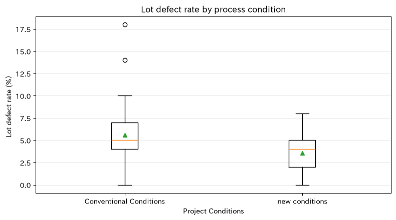
For 180 lots, both conventional and new conditions are operated in parallel, and data is generated from inspecting 100 lots per lot.

• Room temperature, processing speed, and material sources vary by lot
• High temperature, high-speed processing, and supplier C increase the defect rate.
• The new conditions generally reduce the probability of defects and partially mitigate deterioration at high speeds
• Retain both individual data and lot aggregation data

The allocation between old and new is modeled after a fictional parallel exam. In practice, randomization and block management—which do not bias time, equipment, workers, or product types—are more important than analytical methods.

SEED = 20260711
rng = np.random.default_rng(SEED)
n_lots, units_per_lot = 180, 100

lot_id = np.arange(1, n_lots + 1)
new_process = rng.integers(0, 2, n_lots)
temperature = rng.normal(25.0, 3.0, n_lots)
speed = np.clip(rng.normal(100.0, 5.0, n_lots), 88, 112)
supplier_c = rng.binomial(1, 0.30, n_lots)

logit_p = (
    -3.00
    - 0.52 * new_process
    + 0.075 * (temperature - 25)
    + 0.040 * (speed - 100)
    + 0.42 * supplier_c
    - 0.025 * new_process * (speed - 100)
)
defect_probability = expit(logit_p)
defect_matrix = rng.binomial(1, defect_probability[:, None], (n_lots, units_per_lot))

lots = pd.DataFrame({
    "lotID": lot_id,
    "Project Conditions": np.where(new_process == 1, "new conditions", "Conventional Conditions"),
    "New Condition Flag": new_process,
    "room_temperature_c": temperature,
    "machining_speed_piece_per_min": speed,
    "SupplierCflag": supplier_c,
    "number_of_inspections": units_per_lot,
    "number_of_defects": defect_matrix.sum(axis=1),
})
lots["non_performing_rate"] = lots["number_of_defects"] / lots["number_of_inspections"]

unit_df = lots.loc[lots.index.repeat(units_per_lot), [
    "lotID", "Project Conditions", "New Condition Flag", "room_temperature_c",
    "machining_speed_piece_per_min", "SupplierCflag"
]].reset_index(drop=True)
unit_df["bad"] = defect_matrix.reshape(-1)

process_summary = lots.groupby("Project Conditions", sort=False).agg(
    lot_size=("lotID", "size"), number_of_inspections=("number_of_inspections", "sum"),
    number_of_defects=("number_of_defects", "sum"), average_room_temperature_c=("room_temperature_c", "mean"),
    average_machining_speed=("machining_speed_piece_per_min", "mean")
)
process_summary["non_performing_rate"] = process_summary["number_of_defects"] / process_summary["number_of_inspections"]
display(lots.head())
display(process_summary)

fig, ax = plt.subplots()
plot_order = ["Conventional Conditions", "new conditions"]
lot_plot = [lots.loc[lots["Project Conditions"] == x, "non_performing_rate"] * 100 for x in plot_order]
ax.boxplot(lot_plot, tick_labels=plot_order, showmeans=True)
ax.set_title("Lot defect rate by process condition")
ax.set_xlabel("Project Conditions")
ax.set_ylabel("Lot defect rate (%）")
ax.grid(axis="y", alpha=0.3)
plt.tight_layout()
plt.show()

	lotID	Project Conditions	New Condition Flag	room_temperature_C	machining_speed_piece_per_min	SupplierCflag	number_of_inspections	number_of_defects	non_performing_rate
0	1	new conditions	1	26.1386	104.2447	1	100	3	0.03
1	2	Conventional Conditions	0	25.2721	107.1965	0	100	5	0.05
2	3	Conventional Conditions	0	26.6385	103.8079	0	100	5	0.05
3	4	new conditions	1	21.5988	91.5556	1	100	0	0.00
4	5	Conventional Conditions	0	24.5195	106.7708	0	100	8	0.08

	lot_size	number_of_inspections	number_of_defects	Average room temperature_C	average_machining_speed	non_performing_rate
Project Conditions
new conditions	91	9100	325	25.1617	100.2791	0.0357
Conventional Conditions	89	8900	498	24.7362	101.0576	0.0560

---

No.091: What is Hypothesis Testing?

Meaning in Practice

Hypothesis testing measures how much the observed defect rate difference deviates from the criterion of “no difference in process conditions.” This tool evaluates using procedures that align the strength of evidence against random fluctuations, rather than automatic judges for mass production.

Approach to Analysis and Modeling

Let the parent defect rates of the conventional and new conditions be $p_0,p_1$, and the one-sided hypothesis

$$H_0:p_1=p_0,\qquad H_1:p_1<p_0$$

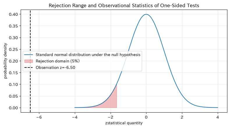
Place. Set the significance level as $alpha=0.05$, and check whether the standardized statistic under the null hypothesis falls within the left-5% rejection range. If you select the direction after checking the data, the error rate will be compromised, so decide whether to choose one side or both sides before the test.

Check with Python

agg = unit_df.groupby("Project Conditions")["bad"].agg(["sum", "count"])
x0, n0 = agg.loc["Conventional Conditions", ["sum", "count"]]
x1, n1 = agg.loc["new conditions", ["sum", "count"]]
p0_hat, p1_hat = x0 / n0, x1 / n1
pooled = (x0 + x1) / (n0 + n1)
se_null = np.sqrt(pooled * (1 - pooled) * (1 / n0 + 1 / n1))
z_score = (p1_hat - p0_hat) / se_null
p_one_sided = norm.cdf(z_score)
critical = norm.ppf(0.05)

test_091 = pd.DataFrame({
    "observation_difference_new-Conventional": [p1_hat - p0_hat], "zstatistical quantity": [z_score],
    "one sidepvalue": [p_one_sided], "5%critical value": [critical],
    "determination": ["Rejection of the null hypothesis" if z_score < critical else "cannot be dismissed"]
})
display(test_091)

z_grid = np.linspace(-4, 4, 500)
fig, ax = plt.subplots()
ax.plot(z_grid, norm.pdf(z_grid), label="Standard normal distribution under the null hypothesis")
ax.fill_between(z_grid, 0, norm.pdf(z_grid), where=z_grid <= critical,
                alpha=0.3, color="tab:red", label="Rejection domain (5%）")
ax.axvline(z_score, color="black", linestyle="--", label=f"Observation z={z_score:.2f}")
ax.set_title("Rejection Range and Observational Statistics of One-Sided Tests")
ax.set_xlabel("zstatistical quantity")
ax.set_ylabel("probability density")
ax.grid(alpha=0.3)
ax.legend()
plt.tight_layout()
plt.show()

	observation_difference_new-Conventional	zstatistical quantity	one sidepvalue	5%critical value	determination
0	-0.0202	-6.4999	4.0192e-11	-1.6449	Rejection of the null hypothesis

Reading the results

The defect rate of the observed new condition is lower than that of the previous condition, and the Z statistic falls within a one-sided 5% rejection range. Based on this data and assumptions, the difference is difficult to explain simply by saying ‘the defect rates between old and new mothers are the same.’ However, rejection does not independently prove that the new conditions are the cause. After confirming the fairness of allocation, measurement methods, time periods, and whether there was any interruption, we connect the scope of improvement and cost to the next decision.

---

No.092: Likelihood Ratio Test

Meaning in Practice

The likelihood ratio test compares the fit of data between a simple model with only a common defect rate between old and new, and a model with defect rates for both old and new. It can be read as a model comparison to see if it is worth adding process conditions to the model.

Approach to Analysis and Modeling

If the log-likelihood of the binomial model is $ell$, the test statistic is

$$G^2=2\{\ell(\hat{p}_0,\hat{p}_1)-\ell(\hat{p}_{\mathrm{pool}})\}$$

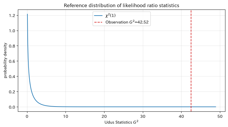
That’s right. In large specimens, under $H_0$, it approaches a chi-square distribution with 1 degree of freedom. Likelihood is not the “probability that the hypothesis is correct,” but rather how consistent the observational data is when parameters are fixed.

Check with Python

def binomial_loglik(x, n, p):
    p = np.clip(p, 1e-12, 1 - 1e-12)
    return x * np.log(p) + (n - x) * np.log1p(-p)

ll_null = binomial_loglik(x0 + x1, n0 + n1, pooled)
ll_alt = binomial_loglik(x0, n0, p0_hat) + binomial_loglik(x1, n1, p1_hat)
lr_stat = 2 * (ll_alt - ll_null)
lr_p = chi2.sf(lr_stat, df=1)
lr_table = pd.DataFrame({
    "Model": ["Common Non-Performing Rate", "Non-performing Rate by New and Old"],
    "Number of parameters": [1, 2], "Maximum log-likelihood": [ll_null, ll_alt]
})
display(lr_table)
display(pd.DataFrame({"Udus Statistics": [lr_stat], "degree of freedom": [1], "pvalue": [lr_p]}))

fig, ax = plt.subplots()
g_grid = np.linspace(0, max(12, lr_stat * 1.15), 500)
ax.plot(g_grid, chi2.pdf(g_grid, 1), label=r"$\chi^2(1)$")
ax.axvline(lr_stat, color="tab:red", linestyle="--", label=f"Observation $G^2$={lr_stat:.2f}")
ax.set_title("Reference distribution of likelihood ratio statistics")
ax.set_xlabel("Udus Statistics $G^2$")
ax.set_ylabel("probability density")
ax.grid(alpha=0.3)
ax.legend()
plt.tight_layout()
plt.show()

	Model	Number of parameters	Maximum log-likelihood
0	Common Non-Performing Rate	1	-3342.9874
1	Non-performing Rate by New and Old	2	-3321.7292

	Udus Statistics	degree of freedom	pvalue
0	42.5165	1	7.0089e-11

Reading the results

The old and new models have higher log-likelihood than the common defect rate model, and the p-value corresponding to the likelihood ratio statistic is smaller. There is statistical evidence for adding process conditions as an explanatory variable. However, improving fit is separate from economic value. The break-even point for new conditions, including equipment costs, speed, yield, and guarantee losses, is used to determine the break-even point.

---

No.093: Wald Certification

Meaning in Practice

The Wald test evaluates whether the estimated improvement is sufficiently large compared to the standard error. Because it is easy to calculate with estimates and standard errors, it is widely used for coefficient evaluation in regression models.

Approach to Analysis and Modeling

The Wald statistic for defect rate difference $d=\hat{p}_1-\hat{p}_0$

$$Z_W=\frac{d}{\sqrt{\hat{p}_1(1-\hat{p}_1)/n_1+\hat{p}_0(1-\hat{p}_0)/n_0}}$$

Let’s say so. The denominator is evaluated as an unconstrained estimate. If the sample is small, the ratio is close to 0 or 1, or the model is close to the boundary, the approximation may be poor.

Check with Python

difference = p1_hat - p0_hat
se_wald = np.sqrt(p1_hat * (1 - p1_hat) / n1 + p0_hat * (1 - p0_hat) / n0)
z_wald = difference / se_wald
p_wald_two = 2 * norm.sf(abs(z_wald))
components = pd.DataFrame({
    "item": ["Dispersion Contributions under New Terms", "Variance Contribution under Conventional Conditions", "standard error"],
    "value": [p1_hat * (1 - p1_hat) / n1, p0_hat * (1 - p0_hat) / n0, se_wald]
})
display(components)
display(pd.DataFrame({
    "Non-performing Rate Difference": [difference], "Wald z": [z_wald], "both sidespvalue": [p_wald_two]
}))

fig, ax = plt.subplots()
labels = ["Conventional Conditions", "new conditions"]
rates = np.array([p0_hat, p1_hat]) * 100
errors = np.array([
    np.sqrt(p0_hat * (1 - p0_hat) / n0),
    np.sqrt(p1_hat * (1 - p1_hat) / n1)
]) * 1.96 * 100
ax.errorbar(labels, rates, yerr=errors, fmt="o", capsize=6, markersize=8)
ax.set_title("Defect rates by process conditionWaldapproximate interval")
ax.set_xlabel("Project Conditions")
ax.set_ylabel("Defect Rate (%）")
ax.grid(axis="y", alpha=0.3)
plt.tight_layout()
plt.show()

	item	value
0	Dispersion Contributions under New Terms	3.7845e-06
1	Variance Contribution under Conventional Conditions	5.9353e-06
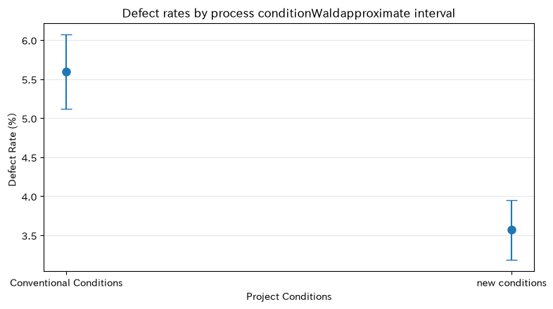
2	standard error	3.1177e-03

	Non-performing Rate Difference	Wald z	both sidespvalue
0	-0.0202	-6.4923	8.4532e-11

Reading the results

The estimated defect rate difference is several times the standard error, and the results of the two-sided test also show the difference. Wald’s test mainly looks at estimates, making correspondence with effect sizes easier to understand, but it is unstable with rarity or small samples. In such cases, exact tests, likelihood methods, and profile likelihood intervals are also considered as candidates.

---

No.094: Score Certification

Meaning in Practice

The Score test examines how strongly the likelihood tilts toward the direction of the difference at the position where no difference is assumed. There are situations where you can consider adding variables without making the entire alternative model estimatory.

Approach to Analysis and Modeling

Generally, scores are the slope of log-likelihood

$$U(\theta)=\frac{\partial \ell(\theta)}{\partial\theta}$$

That’s right. For equivalence of the two ratios, the z-test, which uses the common estimate $hat{p}_{\mathrm{pool}}$ under the null hypothesis as the standard error, corresponds to the score test. Wald is an unconstrained estimate, Score is an estimate under the null hypothesis, and the likelihood ratio differs in the difference between the maximum likelihood between the two.

Check with Python

score_z = difference / np.sqrt(pooled * (1 - pooled) * (1 / n0 + 1 / n1))
score_chi2 = score_z ** 2
score_p = chi2.sf(score_chi2, 1)
comparison = pd.DataFrame({
    "Certification": ["Udobi", "Wald", "Score"],
    "Statistical Measure (Chi-square Scale)": [lr_stat, z_wald ** 2, score_chi2],
    "both sidespvalue": [lr_p, p_wald_two, score_p],
    "Evaluation Position": ["Likelihood difference between constraints and non-constraints", "unconstrained estimate", "Null hypothesis (lower part)"]
})
display(comparison)

fig, ax = plt.subplots()
ax.bar(comparison["Certification"], comparison["Statistical Measure (Chi-square Scale)"],
       color=["tab:blue", "tab:orange", "tab:green"])
ax.axhline(chi2.ppf(0.95, 1), color="tab:red", linestyle="--", label="5%critical value")
ax.set_title("3Comparison of large-sample tests")
ax.set_xlabel("Examination Method")
ax.set_ylabel("Statistics on the Chi-square Scale")
ax.grid(axis="y", alpha=0.3)
ax.legend()
plt.tight_layout()
plt.show()

	Certification	Statistical Measure (Chi-square Scale)	both sidespvalue	Evaluation Position
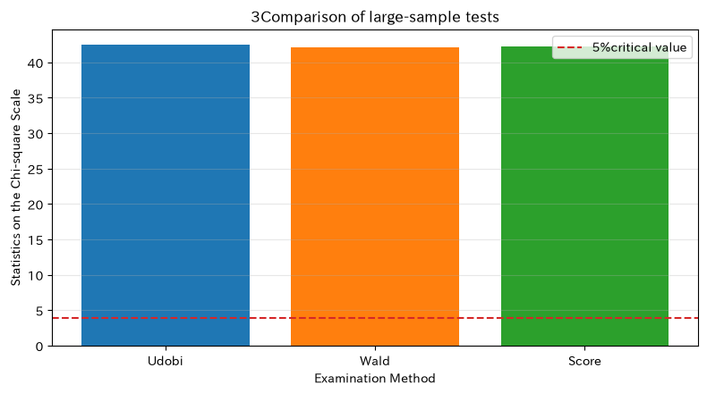
0	Udobi	42.5165	7.0089e-11	Likelihood difference between constraints and non-constraints
1	Wald	42.1500	8.4532e-11	unconstrained estimate
2	Score	42.2485	8.0383e-11	Null hypothesis (lower part)

Reading the results

Since the number of tests and defect rates are far from the boundary this time, the three-test analysis—likelihood ratio, Wald, and Score—is close to the conclusion. Matching is not always guaranteed. If values differ, do not vote by majority vote; instead, check small samples, boundaries, model misdesignation, and numerical optimization, and select the method best suited to the data generation process.

---

No.095: The Meaning of the p-Value

Meaning in Practice

The p-value is neither the “probability that the new condition is ineffective” nor the “probability that this conclusion is wrong.” When the null hypothesis and the analysis procedure are fixed, the probability that results are more extreme than the observed values will occur. In management decisions, the amount of effect and loss are evaluated separately.

Approach to Analysis and Modeling

If the statistic is $T$ and the observed value is $t_{\mathrm{obs}}$, then the two-sided p-values are conceptually

$$p=P_{H_0}(|T|\geq |t_{\mathrm{obs}}|)$$

That’s right. If the null hypothesis is correct and continuous tests are properly used, the p-value will be roughly uniformly distributed. If you repeatedly check and stop at any point or select only the smallest values from multiple comparisons, this property is compromised.

Check with Python

rng_p = np.random.default_rng(SEED + 95)
n_sim = 10_000
sim_x0 = rng_p.binomial(n0, pooled, n_sim)
sim_x1 = rng_p.binomial(n1, pooled, n_sim)
sim_d = sim_x1 / n1 - sim_x0 / n0
sim_z = sim_d / se_null
simulation_p = np.mean(np.abs(sim_z) >= abs(score_z))
display(pd.DataFrame({
    "Theoretical Dual Sidespvalue": [score_p], "Null Distribution Simulationpvalue": [simulation_p],
    "Number of simulations": [n_sim]
}))

fig, ax = plt.subplots()
ax.hist(sim_z, bins=50, density=True, alpha=0.7, color="tab:blue", label="Simulation under the null hypothesisz")
ax.axvline(score_z, color="tab:red", linestyle="--", label=f"Observation z={score_z:.2f}")
ax.axvline(-score_z, color="tab:red", linestyle="--")
ax.set_title("pRepeated distributions under the null hypothesis that creates values")
ax.set_xlabel("zstatistical quantity")
ax.set_ylabel("probability density")
ax.grid(alpha=0.3)
ax.legend()
plt.tight_layout()
plt.show()

	Theoretical Dual Sidespvalue	Null Distribution Simulationpvalue	Number of simulations
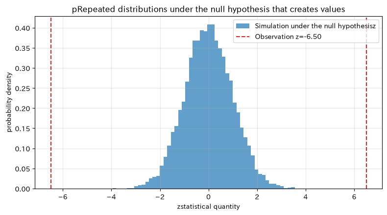
0	8.0383e-11	0.0	10000

Reading the results

In iterations where the defect rate is set for both the old and new models under the null hypothesis, values that are more extreme than the observed statistics rarely appear. This is what a small p-value means. However, p-values do not directly indicate the amount of improvement or the probability of reproduction. It is important to include pre-trial registration, effect size, confidence intervals, measurement quality, and replication, and not to treat the data as merely “small p-values.”

---

No.096: Confidence Interval

Meaning in Practice

Confidence intervals indicate the range within which the improvement is consistent with the data. Not only point estimation, but also pessimism can be seen to see if the investment criteria are met, making decisions about mass production adoption more practical.

Approach to Analysis and Modeling

The approximate 95% confidence interval for the defect rate difference is

$$(\hat{p}_1-\hat{p}_0)\pm 1.96 \sqrt{\frac{\hat{p}_1(1-\hat{p}_1)}{n_1}+\frac{\hat{p}_0(1-\hat{p}_0)}{n_0}}$$

That’s right. Frequently, about 95% of the intervals created when repeating the same procedure cover the true value, which is a nature of the procedure. This does not mean that the probability of a true value entering the fixed interval obtained this time is 95%.

Check with Python

z975 = norm.ppf(0.975)
ci_low, ci_high = difference - z975 * se_wald, difference + z975 * se_wald
# Calculated under the hypothetical condition of 100,000 units per month and 8,000 yen per defective outflow
monthly_volume, loss_per_defect = 100_000, 8_000
avoided_defects_range = (-ci_high * monthly_volume, -ci_low * monthly_volume)
avoided_loss_range = tuple(x * loss_per_defect for x in avoided_defects_range)
ci_table = pd.DataFrame({
    "indicator": ["Defect rate difference (new-Conventional)", "Monthly number of avoidance defects", "monthly_avoidance_loss_yen"],
    "point estimation": [difference, -difference * monthly_volume,
             -difference * monthly_volume * loss_per_defect],
    "95%lower_limit": [ci_low, avoided_defects_range[0], avoided_loss_range[0]],
    "95%upper": [ci_high, avoided_defects_range[1], avoided_loss_range[1]]
})
display(ci_table)

fig, ax = plt.subplots()
ax.errorbar([difference * 100], [0],
            xerr=[[difference * 100 - ci_low * 100], [ci_high * 100 - difference * 100]],
            fmt="o", capsize=7, markersize=8)
ax.axvline(0, color="tab:red", linestyle="--", label="No difference")
ax.set_title("Difference in defect rates between new and old conditions:95%confidence interval")
ax.set_xlabel("Defect rate difference (new condition − Under the previous conditions,%Points)")
ax.set_ylabel("estimated result")
ax.set_yticks([])
ax.grid(axis="x", alpha=0.3)
ax.legend()
plt.tight_layout()
plt.show()

	indicator	point estimation	95%lower_limit	95%upper
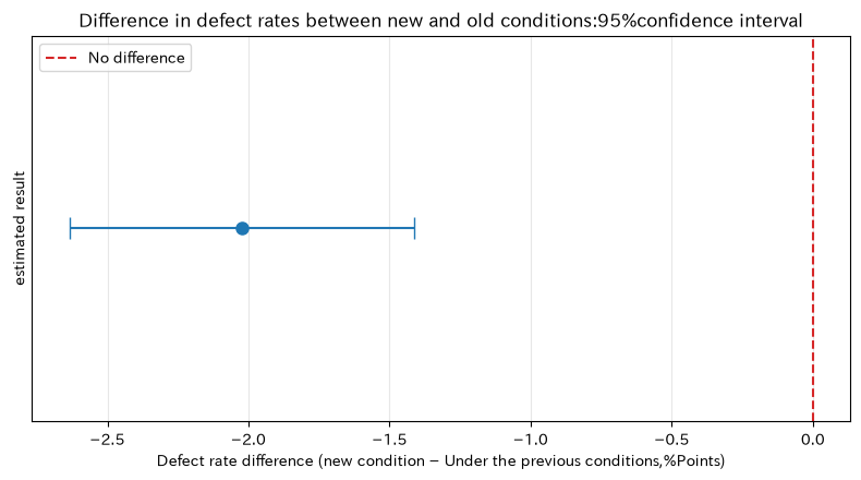
0	Defect rate difference (new-Conventional)	-2.0241e-02	-2.6351e-02	-1.4130e-02
1	Monthly number of avoidance defects	2.0241e+03	1.4130e+03	2.6351e+03
2	monthly_avoidance_loss_jpy	1.6193e+07	1.1304e+07	2.1081e+07

Reading the results

The 95% confidence interval for the defect rate difference is below zero and aligns with the direction of improvement. Furthermore, you can translate fictitious production volumes and loss unit prices into the range of defects and losses to avoid defects. In practice, we compare the pessimistic effect with the implementation costs. Please note that due to uncertainties in loss unit prices and future product composition, the amount range is not limited to statistical intervals alone.

---

No.097: Bayesian Estimation

Meaning in Practice

Bayesian estimation updates prior information about defect rates with the current inspection results and directly calculates the “probability that the defect rate is below what percentage” and “the probability that the new condition is better than the previous one.” You can explicitly integrate information from past tests and similar equipment.

Approach to Analysis and Modeling

If we set the Beta pre-distribution for defect probability $p$ and the binomial distribution for observation defects $X$,

$$p\sim\mathrm{Beta}(a,b),\quad X\mid p\sim\mathrm{Binomial}(n,p)$$ $$p\mid X=x\sim\mathrm{Beta}(a+x,b+n-x)$$

That’s how it works. Here, we use the Jeffreys prior distribution $\mathrm{Beta}(0.5,0.5)$ of weak information for both conditions. The pre-distribution is not hidden; it is included in the sensitivity analysis.

Check with Python

a_prior = b_prior = 0.5
post0 = (a_prior + x0, b_prior + n0 - x0)
post1 = (a_prior + x1, b_prior + n1 - x1)
rng_b = np.random.default_rng(SEED + 97)
draws0 = rng_b.beta(*post0, 100_000)
draws1 = rng_b.beta(*post1, 100_000)

posterior_table = pd.DataFrame({
    "Project Conditions": ["Conventional Conditions", "new conditions"],
    "Post-event average": [draws0.mean(), draws1.mean()],
    "95%Lower limit of the credit range": [np.quantile(draws0, 0.025), np.quantile(draws1, 0.025)],
    "95%Credit Bracket Limit": [np.quantile(draws0, 0.975), np.quantile(draws1, 0.975)]
})
display(posterior_table)
display(pd.DataFrame({
    "P(Defect Rate Under the New Conditions < Conventional Conditions)": [np.mean(draws1 < draws0)],
    "P(1%Improvement over points)": [np.mean(draws0 - draws1 > 0.01)]
}))

p_grid = np.linspace(0.01, 0.08, 500)
fig, ax = plt.subplots()
ax.plot(p_grid * 100, beta.pdf(p_grid, *post0), label="Conventional Conditions")
ax.plot(p_grid * 100, beta.pdf(p_grid, *post1), label="new conditions")
ax.set_title("Post-mortem distribution of defect rates by process condition")
ax.set_xlabel("Mother defect rate (%）")
ax.set_ylabel("posterior probability density")
ax.grid(alpha=0.3)
ax.legend()
plt.tight_layout()
plt.show()

	Project Conditions	Post-event average	95%Lower limit of the credit range	95%Credit Bracket Limit
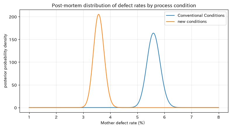
0	Conventional Conditions	0.0560	0.0513	0.0609
1	new conditions	0.0358	0.0320	0.0397

	P(Defect Rate Under the New Conditions < Conventional Conditions)	P(1%Improvement over points)
0	1.0	0.9994

Reading the results

The posterior distribution of the new condition is positioned lower than the previous condition, allowing direct confirmation of the posterior probability where the parent defect rate is lower under the new condition. The probability of “improvement of 1 percentage point or more” can be read as the certainty of meeting the minimum practical effect. However, insufficient randomization and measurement bias do not disappear even when the posterior distribution is narrowed. The validity of the model and data collection is a prerequisite.

---

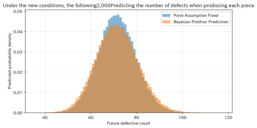
No.098: Bayesian Prediction Distribution

Meaning in Practice

What the quality department wants to know is not only the mother defect rate, but also how many defects might occur next month. Bayesian prediction distributions summarize binomial variability and parameter estimation uncertainties, leading to the design of inspection personnel, rework capacity, and contingency funds.

Approach to Analysis and Modeling

If the future number of defects is $\tilde{X}$, the post-event distribution is

$$p(\tilde{x}\mid x)=\int p(\tilde{x}\mid p)p(p\mid x)\,dp$$

That’s right. In the Beta-Binomial model, you can predict by subtracting the defect rate from the posterior distribution and generating future binomial random numbers from that rate. Compared to binomial predictions that fix point estimation, the parameter uncertainty increases accordingly.

Check with Python

future_n = 2_000
rng_pred = np.random.default_rng(SEED + 98)
posterior_p = rng_pred.beta(*post1, 100_000)
predictive_defects = rng_pred.binomial(future_n, posterior_p)
plug_in_defects = rng_pred.binomial(future_n, p1_hat, 100_000)

pred_table = pd.DataFrame({
    "Methods": ["Bayesian Posthoc Prediction", "Point estimation fixed binomial prediction"],
    "Average number of defects": [predictive_defects.mean(), plug_in_defects.mean()],
    "2.5%point": [np.quantile(predictive_defects, 0.025), np.quantile(plug_in_defects, 0.025)],
    "97.5%point": [np.quantile(predictive_defects, 0.975), np.quantile(plug_in_defects, 0.975)],
    "standard_deviation": [predictive_defects.std(), plug_in_defects.std()]
})
display(pred_table)

fig, ax = plt.subplots()
bins = np.arange(min(predictive_defects.min(), plug_in_defects.min()),
                 max(predictive_defects.max(), plug_in_defects.max()) + 2) - 0.5
ax.hist(plug_in_defects, bins=bins, density=True, alpha=0.55, label="Point Assumption Fixed")
ax.hist(predictive_defects, bins=bins, density=True, alpha=0.55, label="Bayesian Posthoc Prediction")
ax.set_title("Under the new conditions, the following2,000Predicting the number of defects when producing each piece")
ax.set_xlabel("Future defective count")
ax.set_ylabel("Predicted probability density")
ax.grid(alpha=0.3)
ax.legend()
plt.tight_layout()
plt.show()

	Methods	Average number of defects	2.5%point	97.5%point	standard_deviation
0	Bayesian Posthoc Prediction	71.5155	54.0	90.0	9.1363
1	Point estimation fixed binomial prediction	71.4918	56.0	88.0	8.3184

Reading the results

The average of post-mortem predictions is close to the number of predictions expected from the estimated defect rate for new conditions, but the range is broader than fixed-point predictions. This is not only because of the chance of defect occurrence, but also because there is uncertainty in estimating the parent defect rate from finite data. Instead of allocating staff and budgets based solely on averages, you can use 97.5% as a high-load scenario.

---

No.099: Model Selection (AIC/BIC)

Meaning in Practice

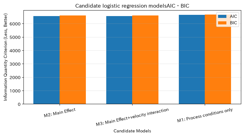
The defect rate depends not only on process conditions but also on room temperature, processing speed, and the source of the material. However, increasing variables and interactions will definitely improve fit to the training data. AIC and BIC compare fit and complexity on the same scale.

Approach to Analysis and Modeling

If the maximum log-likelihood is $\ell_{\max}$, the number of parameters is $k$, and the number of observations is $n$,

$$\mathrm{AIC}=2k-2\ell_{\max},\qquad \mathrm{BIC}=k\log n-2\ell_{\max}$$

That’s right. Choose a smaller model. AIC approximates predicted losses, while BIC punishes complexity more strongly based on assumptions such as a true model among the candidates. Values calculated with different target variables or different data cannot be compared.

Check with Python

y = unit_df["bad"].to_numpy(dtype=float)
new = unit_df["New Condition Flag"].to_numpy(dtype=float)
temp_c = unit_df["room_temperature_c"].to_numpy() - 25
speed_c = unit_df["machining_speed_piece_per_min"].to_numpy() - 100
supplier = unit_df["SupplierCflag"].to_numpy(dtype=float)

design_matrices = {
    "M1: Process conditions only": np.column_stack([np.ones(len(y)), new]),
    "M2: Main Effect": np.column_stack([np.ones(len(y)), new, temp_c, speed_c, supplier]),
    "M3: Main Effect+velocity interaction": np.column_stack([
        np.ones(len(y)), new, temp_c, speed_c, supplier, new * speed_c
    ]),
}

def fit_logistic(X, y):
    def negative_loglik(beta_coef):
        eta = X @ beta_coef
        return np.sum(np.logaddexp(0, eta) - y * eta)
    result = minimize(negative_loglik, np.zeros(X.shape[1]), method="L-BFGS-B")
    return result.x, -result.fun, result.success

model_rows = []
fitted_models = {}
for name, X in design_matrices.items():
    coef, loglik, success = fit_logistic(X, y)
    k = X.shape[1]
    fitted_models[name] = coef
    model_rows.append({
        "Model": name, "Number of parameters": k, "Maximum log-likelihood": loglik,
        "AIC": 2 * k - 2 * loglik,
        "BIC": k * np.log(len(y)) - 2 * loglik,
        "convergence": success
    })
model_comparison = pd.DataFrame(model_rows).sort_values("AIC")
display(model_comparison)

fig, ax = plt.subplots()
x_pos = np.arange(len(model_comparison))
width = 0.36
ax.bar(x_pos - width / 2, model_comparison["AIC"], width, label="AIC")
ax.bar(x_pos + width / 2, model_comparison["BIC"], width, label="BIC")
ax.set_xticks(x_pos, model_comparison["Model"], rotation=12)
ax.set_title("Candidate logistic regression modelsAIC・BIC")
ax.set_xlabel("Candidate Models")
ax.set_ylabel("Information Quantity Criterion (Less, Better)")
ax.grid(axis="y", alpha=0.3)
ax.legend()
plt.tight_layout()
plt.show()

	Model	Number of parameters	Maximum log-likelihood	AIC	BIC	convergence
1	M2: Main Effect	5	-3274.5749	6559.1499	6598.1405	True
2	M3: Main Effect+velocity interaction	6	-3274.1920	6560.3839	6607.1727	True
0	M1: Process conditions only	2	-3321.7292	6647.4583	6663.0546	True

Reading the results

Models that include operating conditions improve the information quantity standards compared to models based solely on process conditions. The value of adding interactions may differ between AIC and BIC, so judgment based on your purpose is necessary. We do not determine causal variables based solely on differences between AIC and BIC; instead, we check hierarchical principles, field knowledge, residual diagnosis, and reproducibility over external periods.

---

No.100: The Intersection of Statistics and Machine Learning

Meaning in Practice

Statistics excel at explaining the effects and uncertainties of process changes, while machine learning excels at risk ranking for the next individual or lot. Quality improvement requires both “why it has changed” and “which is dangerous.”

Approach to Analysis and Modeling

There is no clear boundary between the two, and logistic regression is used for both statistical reasoning and machine learning. The main difference is for evaluation purposes.

• inference: Emphasize coefficients, effect sizes, confidence intervals, assumptions, and identifiability
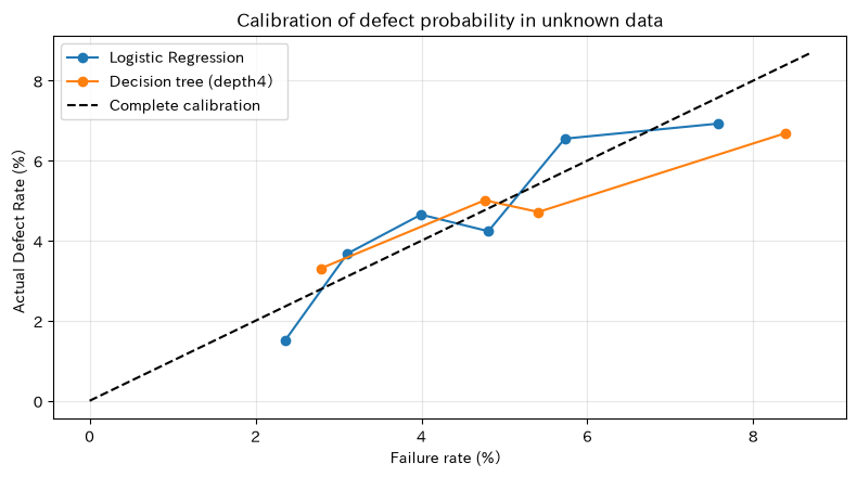
• Prediction: Focus on logarithmic loss of unused data, Brier score, ROC-AUC, and calibration

Because defects are rare, models that are considered “all good” based solely on correct accuracy may be highly rated. We separate and verify the sharpness of probability predictions from calibration.

Check with Python

from sklearn.calibration import calibration_curve
from sklearn.linear_model import LogisticRegression
from sklearn.metrics import accuracy_score, brier_score_loss, log_loss, roc_auc_score
from sklearn.model_selection import train_test_split
from sklearn.tree import DecisionTreeClassifier

feature_cols = ["New Condition Flag", "room_temperature_c", "machining_speed_piece_per_min", "SupplierCflag"]
X_ml = unit_df[feature_cols]
y_ml = unit_df["bad"]
X_train, X_test, y_train, y_test = train_test_split(
    X_ml, y_ml, test_size=0.30, random_state=SEED, stratify=y_ml
)

predictors = {
    "Logistic Regression": LogisticRegression(max_iter=1_000),
    "Decision tree (depth4）": DecisionTreeClassifier(max_depth=4, min_samples_leaf=150, random_state=SEED),
}
metric_rows, probability_predictions = [], {}
for name, estimator in predictors.items():
    estimator.fit(X_train, y_train)
    probability = estimator.predict_proba(X_test)[:, 1]
    probability_predictions[name] = probability
    metric_rows.append({
        "Model": name,
        "Accuracy": accuracy_score(y_test, probability >= 0.5),
        "ROC-AUC": roc_auc_score(y_test, probability),
        "Log loss": log_loss(y_test, probability),
        "Brier score": brier_score_loss(y_test, probability),
    })
metrics = pd.DataFrame(metric_rows)
display(metrics)
print(f"Test Data Defect Rate: {y_test.mean():.4f}")

fig, ax = plt.subplots()
for name, probability in probability_predictions.items():
    observed, predicted = calibration_curve(y_test, probability, n_bins=6, strategy="quantile")
    ax.plot(predicted * 100, observed * 100, marker="o", label=name)
max_rate = max(ax.get_xlim()[1], ax.get_ylim()[1])
ax.plot([0, max_rate], [0, max_rate], linestyle="--", color="black", label="Complete calibration")
ax.set_title("Calibration of defect probability in unknown data")
ax.set_xlabel("Failure rate (%）")
ax.set_ylabel("Actual Defect Rate (%）")
ax.grid(alpha=0.3)
ax.legend()
plt.tight_layout()
plt.show()

	Model	Accuracy	ROC-AUC	Log loss	Brier score
0	Logistic Regression	0.9543	0.6156	0.1819	0.0433
1	Decision tree (depth4）	0.9543	0.5799	0.1835	0.0434

Test data defect rate: 0.0457

Reading the results

Although the accuracy of both models appears high due to fewer defects, that alone does not compare the value of the models. ROC-AUC is for ranking, Log loss and Brier score are for probability prediction, and calibration curves evaluate whether the 5% predicted group is really about 5% defective. For effect explanations, test design and inference models are used; for test prioritization, externally validated predictive models are used; and in the final decision, the costs of false positives and overlooks are reflected at the threshold.

Practical Implications Seen Through Target Exercise

Through No.091 to No.100, it is clear that process change evaluations can be designed in the following four layers.

1. Gather evidence: Hypothesis, one-sided/two-sided, significance level, and number of tests determined before the test
2. Read the size: Shows not only p-values, but also effect size, confidence intervals, and credit intervals
3. Translate into the future: Convert forecast distributions into defective quantities, personnel, loss amounts, and supply risks
4. Choose models according to your purpose: Emphasize assumptions and uncertainties in explanations, and unknown data performance and calibration in forecasting.

The likelihood ratio, Wald, and score evaluate the same question from different perspectives. While similar results with large samples are reassuring, matching the test does not correct biases in the test design. Also, frequency theory and Bayesian reasoning are not adversarial choices but provide different information such as error rate management and decision probability.

In management meetings, not only “significant differences” but also consolidating Defect rate differences, intervals, probability of meeting minimum practical effects, predicted range of defect numbers in the next period, value conversion, assumptions into a single sheet makes it easier to connect technical results to investment decisions.

What is necessary for practical implementation

1. Fix the trial plan before analysis

The main endpoint, null hypothesis, one-sided and two-sided analysis, significance level, number of required tests, exclusion criteria, interim analysis, and minimum practical effect will be listed in the proposal. When trying multiple KPIs or multiple conditions, manage redundancy.

2. Create comparability on the process side

We do not bias old and new conditions toward timing, equipment, varieties, materials, or workers, and if possible, randomize and block the system. Using the same measuring instruments, inspection standards, and sampling methods, we also analyze measurement systems.

3. Turning effect volume into profit and loss

Defect rate differences are converted into disposal, rework, sorting, leakage guarantee, delivery time, and capacity loss. Evaluate return on investment under pessimistic, standard, and optimistic scenarios, including implementation costs, maintenance costs, slowdowns, and side effects.

4. Check Model Assumptions and Sensitivity

Check for intra-lot correlation, overdispersion, time series variation, missing measurements, stop rules, and pre-distribution. If an individual cannot be considered independent, consider the lot as the unit of analysis or consider the robust standard error of hierarchical models and clusters.

5. Separate the verification of inference from prediction

Estimating causal effects requires comparative design, while prediction requires time-sensitive later data or external verification at separate facilities. Predictive models monitor not only identification performance but also calibration, threshold-specific costs, and data changes.

6. Apply rules for decision-making and reassessment

It sets the conditions for “recruitment, additional testing, and postponement,” the approval recipients, the timing of re-evaluation, and the criteria for stopping mass production. Data, code, library versions, analysis plans, and approval records are stored so that the same conclusions can be reproduced.

Conclusion

• Hypothesis testing evaluates how extreme the difference in observation is under the null hypothesis
• The likelihood ratio, Wald, and Score test have different evaluation positions, and large samples tend to yield similar results
• The p-value does not represent the probability that a hypothesis is correct nor the magnitude of the effect
• Confidence intervals indicate the extent to which the data is consistent with the improvement
• Bayesian estimation updates prior information with data and can directly calculate the probability of improvement.
• Bayesian forecast distributions integrate random fluctuations in future defective numbers with estimated uncertainty.
• AIC and BIC compare fit and complexity but do not substitute for judging purpose or external validity
• Statistical inference and machine learning can divide the roles of effect explanation and predicting unknown data.

The value of statistical inference is not in creating significant differences. It involves transforming limited test data into decision-making materials that include the possibility of errors, areas for improvement, future risks, and economic value.

Consultations for Corporations

At Surikoubo, we provide the following support targeting quality, production, and maintenance data from manufacturing industries.

• Statistical test planning and sample size design for process changes and capital investment
• Design of decision rules using p-values, confidence intervals, and Bayesian estimation
• Converting quality KPIs into effective amounts linked to disposal, rework, and warranty losses
• Evaluation of predictive models including AIC, BIC, external validation, and calibration
• Corporate training and analytical prototype development using Python notebooks
• Systematizing the integration of analysis results into regular monitoring and approval workflows

You can consult with us from stages such as “wanting to standardize the way significant differences are read internally,” “designing sample sizes for process tests,” or “wanting to connect PoC accuracy to mass production decisions.”

📩 Contact Us: surikobo.co.jp/contact
Please feel free to consult us first.