Turning sample size into a basis for quality judgment—10 exercises on the extreme limit theorem for manufacturing KPIs

On the manufacturing floor, we assess daily average defect rates and average cycle times to determine process stoppages, additional inspections, and capital investments. However, the average of a few data points tends to be random, and safety-side evaluations without assuming distribution tend to be conservative. This article uses a fictional precision parts factory as a subject and connects No.071〜No.080(Limit theorem) to the determination of required sample numbers, management thresholds, and estimation accuracy.

[!NOTE] This material is a notebook previously used by Surikoubo (or personally by the representative, Kazuyama), and has been reconstructed, edited, and published with the company’s permission.
All data listed is fictional and has no relation whatsoever to real companies, factories, or figures.

Introduction: Practical Challenges in Manufacturing Covered in This Article

The setting is a fictional factory that processes precision shafts for automobiles. The quality assurance department estimates process defect rates from spot checks, while the production management department monitors cycle times and daily losses. At the management meeting, explanations for the following questions are necessary.

• How many lots should be observed to treat the average KPI as a stable value?
• Even if the original data is distorted, is it okay to approximate the sample mean normally?
• Whether standardization and error evaluation are possible even if the population variance is unknown
• In situations where distribution cannot be definitively determined, how much can threshold exceedance be evaluated as safe?
• How to convert errors in defect rate estimates into errors in delivery quantities and quality loss

Common situations on site

At the beginning of the month’s meeting, you may request a process stop by saying “the average of the last 10 lots has deteriorated,” while another report might report that “if the average of 100 lots is average, there is no problem.” Also, only the defect rate of 3% is shared, and the sample size of 100 or 10,000 samples may be omitted.

Even if the average value is the same, the sample size will differ in accuracy. Conversely, using only extremely conservative upper bounds for safety purposes can lead to over-inspection and overstocking. You need to organize what is known about the number of datasets, variables, independence, and variance, and choose a theory that fits your purpose.

Why is this issue so difficult to judge?

Many limit theorems describe properties when the sample size is sufficiently large, but the size of the enough varies depending on the distortion of the original distribution, the weight of the hem, autocorrelation, and the accuracy of the determination. $n=30$ is not a uniform rule that can always be approximated normally.

Furthermore, the inequalities of Chebyshev, Markov, Chernoff, Hoeffding, and others differ in the required assumptions and the sharpness of the upper bound. The upper bound is not the actual probability itself, but a guarantee that “under assumption, it will not exceed this.” A practical focus is to distinguish between guaranteed and predicted values and to evaluate the costs associated with maintainability.

Overview of Exercise covered this time

No.	Theme	Judgment in the manufacturing industry
071	Law of large numbers	Confirm observational surveys until cumulative mean stabilizes
072	central limit theorem	Approximate the error of the sample mean from distorted individual record data
073	Slatsky’s theorem	Replace unknown population standard deviations with sample standard deviations
074	delta method	Convert the error in the defect rate into the error in the required number of inputs
075	Chebyshev’s inequality	Suppressing deviation probability from above using only average and variance
076	Markov’s inequality	Assessing the risk of high costs from non-negative quality loss
077	Chernoff Territory	Evaluate the upper probability of the number of binomial defects exponentially
078	Hoeffding inequality	Linking the mean error of bounded test results to sample size
079	Concentration Inequality	Comparing the assumptions of multiple concentration inequalities and maintainability
080	asymptotic normality	Checking the distribution of defect rate estimators and the accuracy of confidence intervals

Preparing the Python environment

We use NumPy, pandas, SciPy, and Matplotlib. It does not depend on external data, and random number seeds are fixed to 20260711. Theoretical values and simulations are displayed side by side, and approximate, upper bound, and actual measurement frequencies are not confused.

import platform
import sys

import japanize_matplotlib  # noqa: Enable F401 Japanese font
import matplotlib
import matplotlib.pyplot as plt
import numpy as np
import pandas as pd
import scipy
from IPython.display import display
from scipy.stats import binom, norm

SEED = 20260711
rng = np.random.default_rng(SEED)
plt.rcParams["figure.figsize"] = (8, 4.5)
plt.rcParams["axes.axisbelow"] = True

print(f"Python     : {sys.version.split()[0]}")
print(f"NumPy      : {np.__version__}")
print(f"pandas     : {pd.__version__}")
print(f"SciPy      : {scipy.__version__}")
print(f"Matplotlib : {matplotlib.__version__}")
print(f"Platform   : {platform.platform()}")

Python     : 3.13.1
NumPy      : 2.5.1
pandas     : 3.0.3
SciPy      : 1.18.0
Matplotlib : 3.11.0
Platform   : macOS-26.3-arm64-arm-64bit-Mach-O

Creation of Fictional Data

For 2,400 lots, it generates inspection numbers, defect counts, average cycle times, and quality losses. Defect rates involve product differences and daily fluctuations, while quality loss is distributed with long hems to the right. For sections where the subsequent theorem is clearly confirmed, separate iterative simulations with fixed conditions are also conducted.

n_lots = 2_400
products = rng.choice(["ProductsA", "ProductsB", "ProductsC"], n_lots, p=[0.50, 0.30, 0.20])
base_p = pd.Series(products).map({"ProductsA": 0.018, "ProductsB": 0.030, "ProductsC": 0.048}).to_numpy()
inspection_n = rng.choice([80, 100, 120], n_lots, p=[0.2, 0.6, 0.2])
lot_p = np.clip(base_p * rng.lognormal(0, 0.18, n_lots), 0.002, 0.15)
defects = rng.binomial(inspection_n, lot_p)
cycle = rng.lognormal(np.log(61), 0.10, n_lots)
quality_loss = 6_000 + 9_000 * defects + rng.lognormal(np.log(8_000), 0.75, n_lots)

df = pd.DataFrame({
    "lotID": [f"L{i:04d}" for i in range(1, n_lots + 1)],
    "Products": products,
    "number_of_inspections": inspection_n,
    "number_of_defects": defects,
    "non_performing_rate": defects / inspection_n,
    "average_cycle_time_sec": cycle,
    "quality_loss_yen": quality_loss,
})
display(df.head())
display(df.groupby("Products", observed=True).agg(
    lot_size=("lotID", "size"),
    average_defect_rate=("non_performing_rate", "mean"),
    average_cycle_time_sec=("average_cycle_time_sec", "mean"),
    average_quality_loss_yen=("quality_loss_yen", "mean"),
).round(3))

	lotID	Products	number_of_inspections	number_of_defects	non_performing_rate	average_cycle_time_sec	quality_loss_jpy
0	L0001	ProductsA	100	1	0.01	60.847742	18462.889513
1	L0002	ProductsC	100	5	0.05	75.243633	66797.020735
2	L0003	ProductsB	100	3	0.03	62.494952	40788.067078
3	L0004	ProductsB	100	2	0.02	56.958848	31125.459117
4	L0005	ProductsC	100	5	0.05	59.491457	63804.395203

	lot_size	average_defect_rate	average_cycle_time_sec	Average quality loss_jpy
Products
ProductsA	1228	0.018	61.560	33018.239
ProductsB	689	0.030	60.998	44068.843
ProductsC	483	0.048	61.182	59565.582

---

No.071: Law of Large Numbers

Meaning in Practice

The law of large numbers shows that when observations follow the same distribution independently, the sample mean approaches the population mean. Seeing the cumulative average of daily quality loss stabilize helps explain the danger of setting an annual budget based solely on a few days.

Approach to Analysis and Modeling

For an independent and identically distributed random variable $X_1,\ldots,X_n$ with an expected value $E[X]=\mu$, the sample mean

$$\bar{X}_n=\frac{1}{n}\sum_{i=1}^n X_i$$

$n\to\infty$ converges probabilistically to $\mu$. This does not mean that the error in the average will always decrease monotonically; rather, it tends to remain stable over the long term while fluctuating along the way.

Check with Python

x = df["quality_loss_yen"].to_numpy()
running_mean = np.cumsum(x) / np.arange(1, len(x) + 1)
reference_mean = x.mean()
checkpoints = [10, 30, 100, 300, 1_000, 2_400]
lln_table = pd.DataFrame({
    "Number of Observation Lots": checkpoints,
    "cumulative_average_loss_yen": [running_mean[i - 1] for i in checkpoints],
    "difference_from_the_average_over_the_entire_period_pct": [100 * (running_mean[i - 1] / reference_mean - 1) for i in checkpoints],
})
display(lln_table.round(2))

plt.plot(np.arange(1, len(x) + 1), running_mean, label="Cumulative mean")
plt.axhline(reference_mean, color="tab:red", linestyle="--", label="2,400Lot Average")
plt.title("Number of Observed Lots and Cumulative Average Quality Loss")
plt.xlabel("Number of Observation Lots")
plt.ylabel("Cumulative Average Quality Loss (Yen/Lot)")
plt.grid(alpha=0.3)
plt.legend()
plt.tight_layout()
plt.show()

	Number of Observation Lots	cumulative_average_loss_jpy	difference_from_the_average_over_the_entire_period_pct
0	10	45265.58	8.99
1	30	41531.88	-0.00
2	100	41717.51	0.44
3	300	41504.03	-0.07
4	1000	40694.68	-2.02
5	2400	41533.34	-0.00

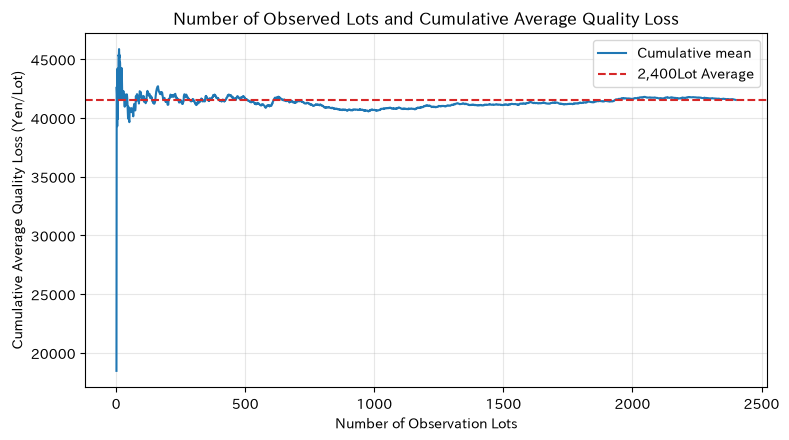
Reading the results

The initial cumulative average moves due to the influence of high-loss lots, but as the number of observations increases, it stabilizes around the 2,400-lot average. However, the law of large numbers does not guarantee that the current average will remain unchanged in the future. If equipment modifications, product compositions, or inspection standards change, the assumption of uniform distribution is undermined. In addition to cumulative averages, it is necessary to manage stratification, time series, and process change points.

---

No.072: Central Limit Theorem

Meaning in Practice

Even if individual cycle times are skewed to the right, the average of multiple lots approaches a normal distribution when the sample size increases. This allows us to explain the margin of error in the weekly average and the margin of capacity planning using a normal approximation.

Approach to Analysis and Modeling

In an independent identically distributed sample with an average $\mu$ and finite variance $\sigma^2$,

$$\frac{\sqrt{n}(\bar{X}_n-\mu)}{\sigma}\xrightarrow{d}N(0,1)$$

This holds. Since the standard deviation of the sample mean is $\sigma/\sqrt{n}$, to halve the error, the sample size should generally be quadrupled.

Check with Python

clt_rng = np.random.default_rng(SEED + 72)
mu_log, sigma_log = np.log(61), 0.28
population_mean = np.exp(mu_log + sigma_log**2 / 2)
population_sd = np.sqrt((np.exp(sigma_log**2) - 1) * np.exp(2 * mu_log + sigma_log**2))
n_reps = 8_000

fig, axes = plt.subplots(1, 3, figsize=(13, 3.8))
clt_rows = []
for ax, n in zip(axes, [5, 30, 100]):
    means = clt_rng.lognormal(mu_log, sigma_log, size=(n_reps, n)).mean(axis=1)
    xs = np.linspace(means.min(), means.max(), 300)
    ax.hist(means, bins=40, density=True, alpha=0.65, color="tab:blue")
    ax.plot(xs, norm.pdf(xs, population_mean, population_sd / np.sqrt(n)), color="tab:red")
    ax.set_title(f"Sample mean (n={n}）")
    ax.set_xlabel("Average cycle time (seconds)")
    ax.set_ylabel("density")
    ax.grid(alpha=0.3)
    clt_rows.append([n, means.mean(), means.std(ddof=1), population_sd / np.sqrt(n)])
plt.tight_layout()
plt.show()
display(pd.DataFrame(clt_rows, columns=["n", "mean of the sample", "Actual measurement of sample meansSD", "theoretical standard error"]).round(3))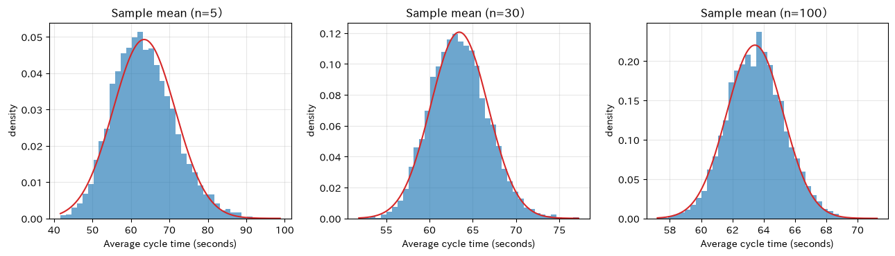

	n	mean of the sample	Actual measurement of sample meansSD	theoretical standard error
0	5	63.403	8.042	8.102
1	30	63.406	3.315	3.308
2	100	63.500	1.829	1.812

Reading the results

Although the original log-normal distribution is skewed to the right, the sample mean distribution approaches a bilaterally symmetrical normal curve as $n$ increases, and the measured SD also matches the theoretical standard error. In small specimens or extremely heavy hem distributions, approximation may be slow. Also, if there is autocorrelation in consecutive lots, the information does not increase as much as the apparent sample size, so the time series structure is also checked.

---

No.073: Slatsky’s Theorem

Meaning in Practice

The central limit theorem yields the base standard deviation $\sigma$, but it is unknown in practice. By Slatsky’s theorem, even if you convert to the sample standard deviation $S$, which is a consistent estimator, it can be explained that large samples approach the same standard normal distribution.

Approach to Analysis and Modeling

$Z_n\xrightarrow{d}Z$, $S_n\xrightarrow{p}\sigma$, then under continuous arithmetic operations, the combined quantities also converge to the corresponding distribution. Therefore,

$$\frac{\sqrt{n}(\bar X_n-\mu)}{S_n}\xrightarrow{d}N(0,1)$$

That’s right. Note that this is not a theorem that asserts precision with finite samples.

Check with Python

sl_rng = np.random.default_rng(SEED + 73)
n, reps = 80, 10_000
samples = sl_rng.lognormal(mu_log, sigma_log, size=(reps, n))
means = samples.mean(axis=1)
s = samples.std(axis=1, ddof=1)
z_known = np.sqrt(n) * (means - population_mean) / population_sd
z_estimated = np.sqrt(n) * (means - population_mean) / s

summary = pd.DataFrame({
    "standardization": ["motherSDusing", "specimenSDusing", "Standard and Regular"],
    "average": [z_known.mean(), z_estimated.mean(), 0],
    "standard_deviation": [z_known.std(ddof=1), z_estimated.std(ddof=1), 1],
    "2.5%point": [np.quantile(z_known, .025), np.quantile(z_estimated, .025), norm.ppf(.025)],
    "97.5%point": [np.quantile(z_known, .975), np.quantile(z_estimated, .975), norm.ppf(.975)],
})
display(summary.round(3))

xs = np.linspace(-4, 4, 300)
plt.hist(z_estimated, bins=50, density=True, alpha=0.65, label="specimenSDStandardization")
plt.plot(xs, norm.pdf(xs), color="tab:red", label="standard normal density")
plt.title("Statistics that replace unknown population standard deviations with sample standard deviations")
plt.xlabel("standardized statistical")
plt.ylabel("density")
plt.grid(alpha=0.3)
plt.legend()
plt.tight_layout()
plt.show()

	standardization	average	standard_deviation	2.5%point	97.5%point
0	motherSDusing	-0.008	1.002	-1.95	1.998
1	specimenSDusing	-0.058	1.027	-2.19	1.873
2	Standard and Regular	0.000	1.000	-1.96	1.960

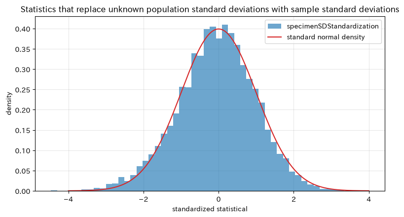
Reading the results

The statistics standardized by sample SD also closely follow the standard normal distribution, with an average of 0 and a standard deviation of 1. This is the theoretical basis for estimating unknown variation from actual results to create standard errors. However, with small samples, substitution error cannot be ignored, so methods suitable for finite samples are prioritized, such as using a t-distribution for the mean of a normal population.

---

No.074: Delta Method

Meaning in Practice

There are situations where you want to report the expected number of inputs to deliver 1,000 good products, not the defect rate itself. The delta method approximately propagates the error in the estimated defect rate to the error of the KPI converted nonlinearly.

Approach to Analysis and Modeling

If $\sqrt{n}(\hat\theta-\theta)\xrightarrow{d}N(0,V)$ is differentiable and $g$ is differentiable,

$$\sqrt{n}\{g(\hat\theta)-g(\theta)\}\xrightarrow{d} N\left(0,\{g'(\theta)\}^2V\right)$$

That’s right. Here, we will $g(p)=1000/(1-p)$ $g'(p)=1000/(1-p)^2$ the defect rate $p$.

Check with Python

delta_rng = np.random.default_rng(SEED + 74)
p_true, n, reps = 0.04, 800, 50_000
p_hat = delta_rng.binomial(n, p_true, reps) / n
required_input = 1_000 / (1 - p_hat)
g_true = 1_000 / (1 - p_true)
se_p = np.sqrt(p_true * (1 - p_true) / n)
delta_se = 1_000 / (1 - p_true) ** 2 * se_p

delta_table = pd.DataFrame({
    "indicator": ["ConversionKPIAverage", "ConversionKPIStandard deviation", "95%lower_limit", "95%upper"],
    "Simulation": [required_input.mean(), required_input.std(ddof=1), *np.quantile(required_input, [.025, .975])],
    "delta method": [g_true, delta_se, g_true - 1.96 * delta_se, g_true + 1.96 * delta_se],
})
display(delta_table.round(2))

plt.hist(required_input, bins=45, density=True, alpha=0.65, label="Simulation")
xs = np.linspace(required_input.min(), required_input.max(), 300)
plt.plot(xs, norm.pdf(xs, g_true, delta_se), color="tab:red", label="Delta Method Normal Approximation")
plt.title("Propagate defect rate estimation errors to the required input quantity")
plt.xlabel("good product1,000Required number of inputs per unit (units)")
plt.ylabel("density")
plt.grid(alpha=0.3)
plt.legend()
plt.tight_layout()
plt.show()

	indicator	Simulation	delta method
0	ConversionKPIAverage	1041.78	1041.67
1	ConversionKPIStandard deviation	7.50	7.52
2	95%lower_limit	1028.28	1026.93
3	95%upper	1056.80	1056.40

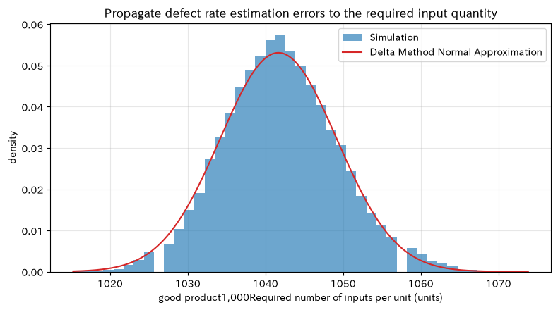
Reading the results

The delta method’s standard error and 95% range are values close to those in iterative simulations. By not only estimating the defect rate points but also adding a range to the required input quantity, you can discuss material arrangements and capacity availability. In regions where the transformation bends sharply, near boundaries, and small samples, normal approximations tend to break down, so bootstraps or direct simulations are compared to this.

---

No.075: Chebyshev’s Inequality

Meaning in Practice

Even if you cannot identify the distribution pattern of process KPIs, knowing the mean and finite variance helps suppress the probability of deviating significantly from the mean. It can be used for safety side evaluations during periods when the basis for distribution assumptions is weak in new processes.

Approach to Analysis and Modeling

For any random variable with an average $\mu$ and standard deviation $\sigma$, if $k>0$ is

$$P(|X-\mu|\ge k\sigma)\le \frac{1}{k^2}$$

That’s right. Instead of assuming little distribution, the upper bound is generally conservative.

Check with Python

loss = df["quality_loss_yen"].to_numpy()
mu_loss, sd_loss = loss.mean(), loss.std(ddof=0)
k_values = np.array([1.5, 2.0, 2.5, 3.0, 4.0])
empirical = np.array([np.mean(np.abs(loss - mu_loss) >= k * sd_loss) for k in k_values])
cheb = 1 / k_values**2
cheb_table = pd.DataFrame({"k": k_values, "Measured Deviation Rate": empirical, "Chebyshev Upper World": cheb})
display(cheb_table.round(4))

plt.plot(k_values, empirical, marker="o", label="Measured Deviation Rate")
plt.plot(k_values, cheb, marker="s", label="Chebyshev Upper World")
plt.title("From the averagekProbability of deviating from the standard deviation or greater")
plt.xlabel("k(Multiple of the standard deviation)")
plt.ylabel("Probability and upper bound")
plt.grid(alpha=0.3)
plt.legend()
plt.tight_layout()
plt.show()

	k	Measured Deviation Rate	Chebyshev Upper World
0	1.5	0.0996	0.4444
1	2.0	0.0450	0.2500
2	2.5	0.0208	0.1600
3	3.0	0.0100	0.1111
4	4.0	0.0025	0.0625

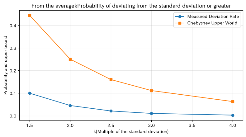
Reading the results

At all thresholds, the actual deviation rate is below the Chebyshev upper bound, but the difference is large, and using the upper bound as a prediction overestimates risk. This inequality is suitable for creating a “minimum guarantee.” In practice, after obtaining sufficient histories, distribution fitting and resampling are used together, and additional inspections and inventory costs due to maintainability are also clearly indicated.

---

No.076: Markov’s Inequality

Meaning in Practice

Non-negative KPIs such as quality loss, downtime, and rework hours can create an upper bound for high costs and long hours beyond the average. It is effective when setting a provisional risk limit on a new line without detailed distribution.

Approach to Analysis and Modeling

For non-negative random variables $X$ and $a>0$,

$$P(X\ge a)\le\frac{E[X]}{a}$$

is Markov’s inequality. Since only non-negativity is used, the range of application is broad, but if the upper bound exceeds 1, it is rounded down to the trivial upper bound 1.

Check with Python

thresholds = np.array([40_000, 60_000, 80_000, 120_000, 180_000])
markov_emp = np.array([(loss >= a).mean() for a in thresholds])
markov_bound = np.minimum(1, mu_loss / thresholds)
markov_table = pd.DataFrame({
    "loss_threshold_yen": thresholds,
    "Actual Over-Measurement Rate": markov_emp,
    "Markov Upper Realm": markov_bound,
    "From the Upper World Perspective1000Maximum number of lots": np.ceil(1_000 * markov_bound).astype(int),
})
display(markov_table.round(4))

plt.plot(thresholds, markov_emp, marker="o", label="Actual Over-Measurement Rate")
plt.plot(thresholds, markov_bound, marker="s", label="Markov Upper Realm")
plt.title("Quality loss threshold exceeding rate and Markov upper bound")
plt.xlabel("Threshold for quality loss (in circles)/Lot)")
plt.ylabel("Excess Probability & Upper Bound")
plt.grid(alpha=0.3)
plt.legend()
plt.tight_layout()
plt.show()

	loss_threshold_jpy	Actual Over-Measurement Rate	Markov Upper Realm	From the Upper World Perspective1000Maximum number of lots
0	40000	0.4483	1.0000	1000
1	60000	0.1721	0.6922	693
2	80000	0.0542	0.5192	520
3	120000	0.0029	0.3461	347
4	180000	0.0000	0.2307	231

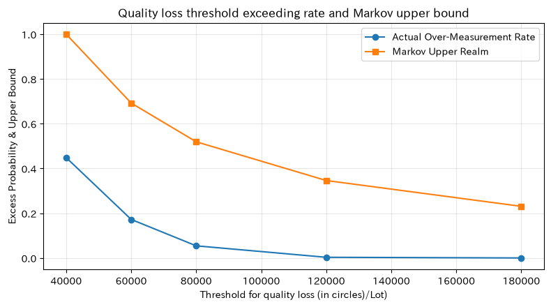
Reading the results

The Markov upper bound certainly exceeds the actual over-measurement rate, but it is quite conservative. The value lies in being able to show an upper limit even when only average losses are shared, and it is not a method for precise forecasting. If KPIs may be negative, they cannot be applied as is. If you use it for a warranty budget, compare the cost difference with methods that add variance or distribution information.

---

No.077: Chernoff Realm

Meaning in Practice

For lots assuming a fixed defect rate, the probability that the number of defects far exceeds the expected value is evaluated exponentially as an upper bound. You can identify risk orders at alarm thresholds without running a full simulation.

Approach to Analysis and Modeling

$X\sim\mathrm{Binomial}(n,p)$, $\mu=np$, and $\delta>0$ The multiplicative Chernoff boundary is

$$P\{X\ge(1+\delta)\mu\}\le \left(\frac{e^\delta}{(1+\delta)^{1+\delta}}\right)^\mu$$

That’s right. Because it uses the exponential moment, it rapidly decreases compared to the general upper bound of just average and variance.

Check with Python

n, p = 1_000, 0.02
mu = n * p
thresholds = np.array([25, 30, 35, 40, 45])
deltas = thresholds / mu - 1
exact_tail = binom.sf(thresholds - 1, n, p)
chernoff = (np.exp(deltas) / (1 + deltas) ** (1 + deltas)) ** mu
chernoff_table = pd.DataFrame({
    "alarm_threshold_number_of_defects": thresholds,
    "How many times higher than expectations?": thresholds / mu,
    "Exact Probability of the Binomial Distribution": exact_tail,
    "Chernoffupper realm": chernoff,
})
display(chernoff_table)

plt.semilogy(thresholds, exact_tail, marker="o", label="Exact Probability of the Binomial Distribution")
plt.semilogy(thresholds, chernoff, marker="s", label="Chernoffupper realm")
plt.title("Upper probability of lot defect quantity")
plt.xlabel("Alarm threshold (number of defects)/1,000Individual)")
plt.ylabel("Excess Probability and Upper Bound (Logarithmic Line)")
plt.grid(alpha=0.3, which="both")
plt.legend()
plt.tight_layout()
plt.show()

	alarm_threshold_number_of_defects	How many times higher than expectations?	Exact Probability of the Binomial Distribution	Chernoffupper realm
0	25	1.25	1.545154e-01	0.560689
1	30	1.50	2.069652e-02	0.114870
2	35	1.75	1.326559e-03	0.010188
3	40	2.00	4.339876e-05	0.000441
4	45	2.25	7.717810e-07	0.000010

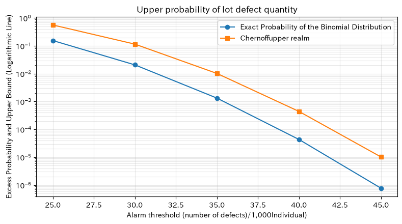
Reading the results

The farther the alarm threshold moves from the 20 expected defects, the exponential decrease in exact probability and Chernoff upper bound. Although the upper bound is larger than the exact probability, it can quickly evaluate the minimal probability digits. However, it is necessary to assume that defects in each individual are independent and have a certain probability. In processes where defects occur frequently due to equipment abnormalities, the binomial model itself tends to be underestimated, so overdispersion and intra-lot correlations are examined.

---

No.078: Hoeffding’s Inequality

Meaning in Practice

The 0/1 data for good or defective products always falls within $[0,1]$. Using the Hoeffding inequality, the probability that the sample defect rate deviates by a certain amount from the true defect rate can be linked to the sample size without using the shape of the population distribution or population variance.

Approach to Analysis and Modeling

About independent $X_i\in[0,1]$,

$$P(|\bar X-E[\bar X]|\ge\varepsilon)\le2\exp(-2n\varepsilon^2)$$

That’s right. If the right-hand side is set to an allowable risk of $\alpha$ or less, you can design a distribution-independent sample size of $n\ge\log(2/\alpha)/(2\varepsilon^2)$.

Check with Python

hf_rng = np.random.default_rng(SEED + 78)
p, eps, reps = 0.03, 0.02, 80_000
n_values = np.array([500, 1_000, 2_000, 5_000, 10_000])
empirical = []
for n in n_values:
    phat = hf_rng.binomial(n, p, reps) / n
    empirical.append(np.mean(np.abs(phat - p) >= eps))
hoeffding = np.minimum(1, 2 * np.exp(-2 * n_values * eps**2))
hf_table = pd.DataFrame({"number_of_inspections_n": n_values, "Measurement error excess rate": empirical, "Hoeffdingupper realm": hoeffding})
display(hf_table)

plt.semilogy(n_values, np.maximum(empirical, 1 / reps), marker="o", label="Measurement error excess rate")
plt.semilogy(n_values, hoeffding, marker="s", label="Hoeffdingupper realm")
plt.title("Sample defect rate from true value2Probability of points being off or more")
plt.xlabel("number_of_inspections n")
plt.ylabel("Probability and upper bound (logarithmic line)")
plt.grid(alpha=0.3, which="both")
plt.legend()
plt.tight_layout()
plt.show()

alpha = 0.05
n_required = int(np.ceil(np.log(2 / alpha) / (2 * eps**2)))
print(f"error±{eps:.1%}to95%Guaranteed by the aboveHoeffdingSample size: {n_required:,}units")

	number_of_inspections_n	Measurement error excess rate	Hoeffdingupper realm
0	500	0.010700	1.000000
1	1000	0.000375	0.898658
2	2000	0.000000	0.403793
3	5000	0.000000	0.036631
4	10000	0.000000	0.000671

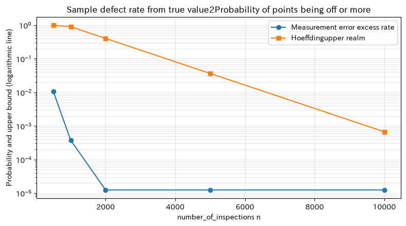
Hoeffding Sample Size: 4,612 specimens with a guaranteed margin of error ± 2.0% and over 95%

Reading the results

Along with the sample size, both the measured error rate and the upper bound decrease. Hoeffding sample size does not use the true defect rate, so it can be designed at process startup, but it is conservative for low-defect processes. If there is autocorrelation in continuous production, random selection of test targets, or measurement errors, even if the sample size is formally met, the guarantee assumption is compromised.

---

No.079: Concentration Inequality

Meaning in Practice

The concentration inequality is a general term for the group of inequalities that guarantee how much the sample mean, etc., is concentrated around the expected value. Even with the same quality data, depending on how reliable the average, variance, and value range is, use different methods such as Chebyshev, Hoeffding, Bernstein, and others.

Approach to Analysis and Modeling

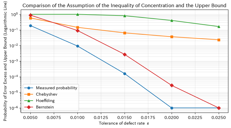
Define the two-sided Bernstein-type upper bound for the mean of independent Bernoulli variables

$$P(|\bar X-p|\ge\varepsilon)\le 2\exp\left\{-\frac{n\varepsilon^2}{2p(1-p)+2\varepsilon/3}\right\}$$

Let’s say so. Because it uses distributed information, it may be sharper than Hoeffding, which uses only the range. On the other hand, Chebyshev does not demand independence or boundaries, but rather a loose upper boundary.

Check with Python

p, n = 0.03, 2_000
eps_values = np.array([0.005, 0.010, 0.015, 0.020, 0.025])
ci_rng = np.random.default_rng(SEED + 79)
phat = ci_rng.binomial(n, p, 200_000) / n
emp = np.array([np.mean(np.abs(phat - p) >= e) for e in eps_values])
cheb = np.minimum(1, p * (1 - p) / (n * eps_values**2))
hoeff = np.minimum(1, 2 * np.exp(-2 * n * eps_values**2))
bern = np.minimum(1, 2 * np.exp(-n * eps_values**2 / (2 * p * (1 - p) + 2 * eps_values / 3)))

concentration = pd.DataFrame({
    "allowable_error_eps": eps_values,
    "Measured probability": emp,
    "Chebyshev": cheb,
    "Hoeffding": hoeff,
    "Bernstein": bern,
})
display(concentration)

for col, marker in [("Measured probability", "o"), ("Chebyshev", "s"), ("Hoeffding", "^"), ("Bernstein", "D")]:
    plt.semilogy(eps_values, np.maximum(concentration[col], 1e-6), marker=marker, label=col)
plt.title("Comparison of the Assumption of the Inequality of Concentration and the Upper Bound")
plt.xlabel("Tolerance of defect rate ε")
plt.ylabel("Probability of Error Excess and Upper Bound (Logarithmic Line)")
plt.grid(alpha=0.3, which="both")
plt.legend()
plt.tight_layout()
plt.show()

	allowable_error_eps	Measured probability	Chebyshev	Hoeffding	Bernstein
0	0.005	0.189615	0.582000	1.000000	8.874345e-01
1	0.010	0.009295	0.145500	1.000000	9.162047e-02
2	0.015	0.000160	0.064667	0.813139	2.725528e-03
3	0.020	0.000000	0.036375	0.403793	2.780068e-05
4	0.025	0.000000	0.023280	0.164170	1.121754e-07

Reading the results

All upper bounds have higher or higher measured probabilities, but generally, the more information you use, the sharper the upper bound becomes. Chebyshev has fewer assumptions, Hoeffding uses range and independence, Bernstein uses further variance—this is an exchange relationship. Instead of selecting the smallest number, select within the range that the field data can explain as meeting assumptions, and report guarantee values, experience frequency, and model predictions in separate columns.

---

No.080: Asymptotic Normality

Meaning in Practice

Many estimates approach a normal distribution around true values as the sample size increases. By confirming this property of the most likely estimator of the defect rate $\hat p$, we can understand the basis and limitations for using normal approximation for confidence intervals and inter-plant comparisons of large samples.

Approach to Analysis and Modeling

The maximum likelihood estimate for the Bernoulli sample is $\hat p=\bar X$,

$$\sqrt{n}(\hat p-p)\xrightarrow{d}N\{0,p(1-p)\}$$

That’s right. Therefore, $\hat p$ approximates $N\{p,p(1-p)/n\}$. However, with low defect rates and small samples, zero defects occur frequently, and symmetrical Wald intervals may become inappropriate.

Check with Python

an_rng = np.random.default_rng(SEED + 80)
p, reps = 0.03, 50_000
rows = []
fig, axes = plt.subplots(1, 3, figsize=(13, 3.8))
for ax, n in zip(axes, [50, 500, 5_000]):
    phat = an_rng.binomial(n, p, reps) / n
    z = np.sqrt(n) * (phat - p) / np.sqrt(p * (1 - p))
    se_hat = np.sqrt(phat * (1 - phat) / n)
    lower, upper = phat - 1.96 * se_hat, phat + 1.96 * se_hat
    coverage = np.mean((lower <= p) & (p <= upper))
    rows.append([n, np.mean(phat == 0), z.mean(), z.std(ddof=1), coverage])
    ax.hist(z, bins=45, density=True, alpha=0.65)
    xs = np.linspace(-4, 4, 300)
    ax.plot(xs, norm.pdf(xs), color="tab:red")
    ax.set_title(f"Standardized defect rate (n={n}）")
    ax.set_xlabel("Standardized estimation error")
    ax.set_ylabel("density")
    ax.grid(alpha=0.3)
plt.tight_layout()
plt.show()

asymptotic_table = pd.DataFrame(rows, columns=["number_of_inspections_n", "bad0Transaction rate", "Mean of Normalization Error", "of normalization errorSD", "Wald95%Interval coverage rate"])
display(asymptotic_table.round(4))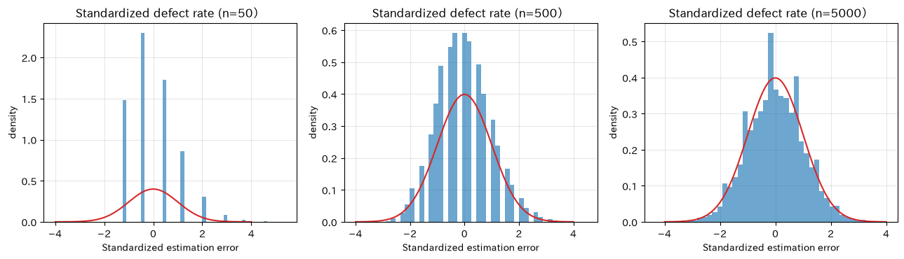

	number_of_inspections_n	bad0Transaction rate	Mean of Normalization Error	of normalization errorSD	Wald95%Interval coverage rate
0	50	0.2181	-0.0040	0.9973	0.7812
1	500	0.0000	0.0046	1.0025	0.9233
2	5000	0.0000	0.0038	0.9972	0.9462

Reading the results

$n=50$ has many defects with zero defects, resulting in a discrete distribution and zero estimated standard error, resulting in insufficient coverage in the Wald section. As $n$ increases, the normalization error approaches the standard normal distribution, and the coverage rate approaches a nominal 95%. For low defect rates and small samples, Wilson intervals and exact methods are used to check the expected number of defects $np$ before judging that a large sample is a normal approximation.

Practical Implications Seen Through Target Exercise

From No.071 to No.080, the following four layers are required to determine manufacturing KPIs.

1. Check Stability: Not only expecting the law of large numbers, but also visualizing cumulative means, stratification, and changes
2. Quantifying estimation errors: Using the central limit theorem, Slatsky, and delta methods, convert point estimation into standard error and decision KPI width.
3. Separating Guarantees from Forecasts: The upper bound of the concentration inequality is not a true probability. The fewer assumptions, the more maintainable it is.
4. Checking finite specimens: Before using asymptotic theory, examine distortion, hem, low incidence rate, autocorrelation, and effective sample size.

The sample size is determined not by “large or small” but by tolerance of error, misjudgment cost, and whether it is sufficient for the process structure.

What is necessary for practical implementation

1. Fix the observation unit and denominator

Whether an individual, lot, day, or equipment is counted as one observation, the denominator of the defect rate, handling of re-inspected items, and the identification of missing or measurement errors are recorded in the data dictionary.

2. Examine the Assumption of Independent and Isometric Distribution

We check time series plots and autocorrelations, stratification by equipment, products, materials, and work zones, as well as process change history. If consecutive lots are correlated, evaluate effective sample sizes and block units.

3. Agree on allowable margins and misjudgment costs

False alarms for process stoppages, missed abnormalities, additional inspections, and delivery delays are converted into amounts and labor to determine the required confidence level and sample size.

4. Operate separately by upper bound, approximate, and actual performance

The report displays the theoretical boundary, model-based estimated probabilities, and past performance excess rates separately, while retaining the assumptions used, target periods, and recalculation conditions. Even after implementation, coverage rates and alarm frequency are monitored and thresholds are updated.

Conclusion

• The law of large numbers supports the stability of cumulative means, but does not guarantee process variation or dependency
• By the central limit theorem, even distorted individual sheets can be normally approximated to the mean of large specimens
• Slatsky’s theorem and delta method support the permutation of unknown variance and the evaluation of errors after KPI transformations
• Chebyshev, Markov, Chernoff, Hoeffding, and others suppress probability from above under different assumptions
• The values of the concentration inequality are not predictive probabilities but guarantee bounds, and maintainability also becomes a cost
• Asymptotic normality is useful, but for low defect rates and small samples, methods for finite samples are chosen

The limit theorem is not a slogan of “as long as there’s more data, it’s fine.” Only by clearly stating what assumptions, what errors to tolerate, and which decisions to adhere to will it become a tool for quality assurance and production management.

Consultations for Corporations

At Suri Kobo, we support everything from organizing data definitions in manufacturing to organizing data definitions, statistical models, simulations, in-house training using Python notebooks, and operational design for quality control, production KPIs, sampling inspections, process capabilities, and anomaly detection.

You can consult from stages such as “explaining the basis for the number of inspections,” “showing the margin of error in average KPIs at management meetings,” or “statistically redesigning existing control limits and alarm thresholds.”

📩 Contact Us: surikobo.co.jp/contact
Please feel free to consult us first.