How to Estimate Failure, Quality, and Maintenance Time—10 Continuous Distribution Options Used in Manufacturing

Overview

The dimensions, waiting times, repair times, and lifespans observed at the manufacturing site show different distribution patterns even for the same “continuous quantity.” In this article, using a fictional precision parts factory as a subject, we will examine the uniform distribution, normal distribution, exponential distribution, gamma distribution, beta distribution, chi-square distribution, t-distribution, F distribution, log-normal distribution, and Weibull distribution using Python.

The goal is not to memorize distribution names. It is about organizing which distributions to use and under what assumptions in decision-making, such as specification rates, preventive maintenance cycles, repair personnel, uncertainty in small data, and variation differences between equipment.

[!NOTE] This material is a notebook previously used by Surikoubo (or personally by the representative, Kazuyama), and has been reconstructed, edited, and published with the company’s permission.
All data listed is fictional and has no relation whatsoever to real companies, factories, or figures.

Introduction: Practical Challenges in Manufacturing Covered in This Article

This time, the setting is a fictional factory that processes precision shafts. The quality assurance department manages the compliance rate for an outer diameter of 20.00 mm and a standard of 19.95–20.05 mm, while the maintenance department develops maintenance plans based on sudden breakdowns and repair times. The questions administrators want to answer are as follows.

• From process capability, how much non-standard issues are likely to occur?
• Is the equipment that has been running for a long time since the last breakdown prone to immediate breakdown?
• How to estimate the time to complete repairs and the long lifespan of parts
• When there is only a small sample, how much can mean and variance be trusted?
• Is there a meaningful practical difference between Equipment A and Equipment B?

Continuous distribution is a common language that expresses these questions not just as “means,” but as probability, quantiles, intervals, and risks.

Common situations on site

At monthly meetings, the average outer diameter, average repair time, and average interval between failures are presented in a single table. However, even if the average is the same, decision-making is not the same.

• The outer diameter is almost symmetrical around the target value, but the repair time is longer on the right side
• The interval between failures is between the contingent failure period and the wear failure period, and the failure rate changes differently over elapsed time
• New equipment has a small sample size and significant uncertainty in the estimates themselves.
• Since it is impossible to test all people, randomization of testing locations and times is necessary.

Simply reporting the same mean and standard deviation does not compare the probabilities of out-of-stock, stoppages, or quality leaks.

Why is this issue so difficult to judge?

First, the selection of distribution involves assumptions about the mechanism of development. Dimensions where many minute factors are added are candidates for the normal distribution, but the gamma distribution is natural for the completion time, which takes only positive values and sums the time required for multiple steps.

Second, fit into the theoretical distribution and usefulness for decision-making are not the same. Even if the histograms are similar, underestimating the probability of the hem will lead to a shortage of maintenance items and personnel. Mixing equipment, products, and failure modes undermines the very assumption of a single distribution.

Third, there is sampling error in the estimates. The uncertainty of the mean is represented by the t-distribution, the variance uncertainty is represented by the chi-square distribution, and the variance ratio between two groups is represented by the F distribution. Rather than definitively determining equipment differences based solely on point estimation, it is necessary to judge based on both the section and the assumptions.

Overview of Exercise covered this time

No.	continuous distribution	Key Challenges in Manufacturing
051	uniform distribution	Whether the examination location is chosen without bias
052	normal distribution	How to estimate the dimensional compliance ratio
053	exponential distribution	How to handle wait times for accidental breakdowns
054	gamma distribution	How to estimate the total time for multiple tasks
055	Beta distribution	How to express the uncertainty of the defect rate?
056	chi-square distribution	How to evaluate the estimation error of process variance
057	t-distribution	How to estimate the population mean using few-based measurements
058	F distribution	2. How to compare the distribution of equipment
059	lognormal distribution	How to plan the repair time for pulling the hem to the right
060	Weibull distribution	How to design lifespan and maintenance cycles, including wear,

For each distribution, we explain not only the form of the probability density function but also assumptions, verification using Python, and considerations when converting output into decision-making.

Preparing the Python environment

Reproduce fictitious data with NumPy, aggregate it with pandas, calculate probability distributions and intervals with SciPy, and visualize it with matplotlib. Seaborn and external data are not used. Random seed numbers are fixed.

import sys

import matplotlib
import matplotlib.pyplot as plt
import numpy as np
import pandas as pd
import scipy
from IPython.display import display
from scipy import stats

import japanize_matplotlib  # Enable Japanese display of matplotlib

SEED = 20260711
rng = np.random.default_rng(SEED)

pd.set_option("display.max_columns", 20)
pd.set_option("display.float_format", lambda x: f"{x:,.4f}")

print(f"Python     : {sys.version.split()[0]}")
print(f"NumPy      : {np.__version__}")
print(f"pandas     : {pd.__version__}")
print(f"SciPy      : {scipy.__version__}")
print(f"matplotlib : {matplotlib.__version__}")
print(f"random seed: {SEED}")

Python     : 3.13.1
NumPy      : 2.5.1
pandas     : 3.0.3
SciPy      : 1.18.0
matplotlib : 3.11.0
random seed: 20260711

Creation of Fictional Data

For analysis, we create the following four types of data.

1. Quality Measurement: Outer diameters of 300 precision shafts machined by Equipment A and B
2. Interval of failures: 300 breakdown intervals assuming accidental failures
3. Restoration Work: Total time spent on four processes—diagnosis, parts replacement, adjustment, and confirmation—250 cases
4. Lifespan and Repairs: 400 parts lifespan including wear and 250 long repair times on the right hem

The distribution at the time of generation is known to compare theoretical values with values obtained from samples. In practice, we separately handle failure mode stratification, distribution fit diagnosis, and handling of cutoff data.

# Quality: Outer diameter data with varying averages and variations for each facility
n_per_machine = 300
quality_df = pd.DataFrame({
    "equipment": np.repeat(["equipmentA", "equipmentB"], n_per_machine),
    "outer_diameter_mm": np.concatenate([
        rng.normal(20.000, 0.018, n_per_machine),
        rng.normal(20.006, 0.027, n_per_machine),
    ]),
})
quality_df["Within the standard"] = quality_df["outer_diameter_mm"].between(19.95, 20.05)

# Inspection & Maintenance: Location, Breakdown Interval, Four Recovery Steps, Repair Time, Wear Life
inspection_df = pd.DataFrame({"inspection_position_on_the_coil_m": rng.uniform(0, 100, 500)})
failure_df = pd.DataFrame({"interval_between_accidental_failures_h": rng.exponential(96, 300)})
task_times = rng.exponential(0.8, size=(250, 4))
recovery_df = pd.DataFrame(task_times, columns=["diagnostic_h", "exchange_h", "adjustment_h", "confirmation_h"])
recovery_df["total_recovery_h"] = recovery_df.sum(axis=1)
repair_df = pd.DataFrame({"repair_time_h": rng.lognormal(np.log(2.5), 0.65, 250)})
life_df = pd.DataFrame({"component_lifespan_h": 1200 * rng.weibull(1.8, 400)})

quality_summary = quality_df.groupby("equipment").agg(
    measurement_quantity=("outer_diameter_mm", "size"),
    average_outer_diameter_mm=("outer_diameter_mm", "mean"),
    standard_deviation_mm=("outer_diameter_mm", "std"),
    rate_within_the_standard=("Within the standard", "mean"),
)
display(quality_summary)

data_summary = pd.DataFrame({
    "Data": ["Examination Location", "interval_between_accidental_failures", "Total recovery time", "repair_time", "component_lifespan"],
    "number_of_cases": [len(inspection_df), len(failure_df), len(recovery_df), len(repair_df), len(life_df)],
    "average": [inspection_df.iloc[:, 0].mean(), failure_df.iloc[:, 0].mean(),
           recovery_df["total_recovery_h"].mean(), repair_df.iloc[:, 0].mean(), life_df.iloc[:, 0].mean()],
    "median": [inspection_df.iloc[:, 0].median(), failure_df.iloc[:, 0].median(),
            recovery_df["total_recovery_h"].median(), repair_df.iloc[:, 0].median(), life_df.iloc[:, 0].median()],
    "Unit": ["m", "h", "h", "h", "h"],
})
display(data_summary.round(3))

	measurement_quantity	average_outer_diameter_mm	standard_deviation_mm	rate_within_the_standard
equipment
equipmentA	300	19.9999	0.0189	0.9933
equipmentB	300	20.0069	0.0260	0.9600

	Data	number_of_cases	average	median	Unit
0	Examination Location	500	47.4910	46.2350	m
1	interval_between_accidental_failures	300	101.9570	69.6000	h
2	Total recovery time	250	3.1670	2.8150	h
3	repair_time	250	3.2540	2.4820	h
4	component_lifespan	400	1,030.8990	941.3880	h

---

No.051: Uniform Distribution

Meaning in Practice

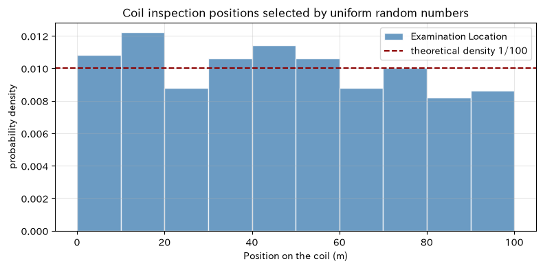
When a single inspection position is randomly selected from a 100 m coil, all positions have the same selection opportunity in a uniformly distributed design. If you only measure near the front, you may miss abnormalities at the end of the wind. Uniform random numbers are used as A system that fairly distributes testing opportunities across space and time, not assuming “quality values are uniform.”

Approach to Analysis and Modeling

The probability density of a continuous uniform distribution over interval $a\le x\le b$ is

$$f(x)=\frac{1}{b-a}, \qquad E[X]=\frac{a+b}{2}, \qquad \mathrm{Var}(X)=\frac{(b-a)^2}{12}$$

That’s right. The probability of choosing 20–40 m is $(40-20)/(100-0)=0.2$ relative to the section length. The probability of the endpoint is exactly zero, but the interval has a positive probability.

Check with Python

positions = inspection_df["inspection_position_on_the_coil_m"]
segment_rate = positions.between(20, 40).mean()
uniform_result = pd.DataFrame({
    "indicator": ["specimen mean(m)", "theoretical mean(m)", "20〜40msample ratio", "20〜40mTheoretical probability"],
    "value": [positions.mean(), 50.0, segment_rate, 0.2],
})
display(uniform_result.round(4))

fig, ax = plt.subplots(figsize=(8, 4))
ax.hist(positions, bins=10, range=(0, 100), density=True,
        color="steelblue", edgecolor="white", alpha=0.8, label="Examination Location")
ax.axhline(1 / 100, color="darkred", linestyle="--", label="theoretical density 1/100")
ax.set_title("Coil inspection positions selected by uniform random numbers")
ax.set_xlabel("Position on the coil (m)")
ax.set_ylabel("probability density")
ax.grid(alpha=0.3)
ax.legend()
plt.tight_layout()
plt.show()

	indicator	value
0	specimen mean(m)	47.4910
1	theoretical mean(m)	50.0000
2	20〜40msample ratio	0.1940
3	20〜40mTheoretical probability	0.2000

Reading the results

The 500 inspection locations are distributed roughly evenly throughout the entire section, and the sample ratio of 20–40 m is close to the theoretical value of 0.2. However, since the sample size is finite, the height of each bottle is not perfectly aligned. In practice, we not only create random numbers but also audit whether there are times when you can’t choose from stops or setups, and whether the selected positions have been replaced due to site circumstances. If periodic abnormalities are suspected, consider not only simple random sampling but also stratified sampling.

---

No.052: Normal Distribution

Meaning in Practice

Machining dimensions can sometimes be approximated by a thick, symmetrical normal distribution near the center, when many small factors such as temperature, tool condition, material, and measurement error act additively. Since the probability of non-standard calculations can be calculated from the mean and standard deviation, it is useful for estimating process capability and inspection load.

Approach to Analysis and Modeling

The density of the normal distribution with mean $\mu$ and standard deviation $\sigma$ is

$$f(x)=\frac{1}{\sqrt{2\pi}\sigma} \exp\left\{-\frac{(x-\mu)^2}{2\sigma^2}\right\}.$$

The probability of falling into the lower limit LSL and upper limit USL is determined using the cumulative distribution function $\Phi$ of the standard normal distribution.

$$P(\mathrm{LSL}\le X\le\mathrm{USL}) =\Phi\!\left(\frac{\mathrm{USL}-\mu}{\sigma}\right) -\Phi\!\left(\frac{\mathrm{LSL}-\mu}{\sigma}\right)$$

It can be expressed as such. Here, we will substitute the sample mean and sample standard deviation for Equipment B.

Check with Python

lsl, usl = 19.95, 20.05
x_b = quality_df.loc[quality_df["equipment"] == "equipmentB", "outer_diameter_mm"]
mu_hat, sigma_hat = x_b.mean(), x_b.std(ddof=1)
predicted_yield = stats.norm.cdf(usl, mu_hat, sigma_hat) - stats.norm.cdf(lsl, mu_hat, sigma_hat)
observed_yield = x_b.between(lsl, usl).mean()

display(pd.DataFrame({
    "average_outer_diameter_mm": [mu_hat], "standard_deviation_mm": [sigma_hat],
    "Rate within the standard by normal distribution": [predicted_yield], "Observation Rate Within Standards": [observed_yield],
}).round(4))

grid = np.linspace(19.90, 20.10, 500)
fig, ax = plt.subplots(figsize=(8, 4))
ax.hist(x_b, bins=24, density=True, alpha=0.65, color="slateblue",
        edgecolor="white", label="equipmentBMeasurement values")
ax.plot(grid, stats.norm.pdf(grid, mu_hat, sigma_hat), color="darkred", label="estimated normal density")
ax.axvline(lsl, color="black", linestyle="--", label="specification limit")
ax.axvline(usl, color="black", linestyle="--")
ax.set_title("equipmentBOuter diameter distribution and specification limits")
ax.set_xlabel("outer_diameter (mm)")
ax.set_ylabel("probability density")
ax.grid(alpha=0.3)
ax.legend()
plt.tight_layout()
plt.show()

	average_outer_diameter_mm	standard_deviation_mm	Rate within the standard by normal distribution	Observation Rate Within Standards
0	20.0069	0.0260	0.9365	0.9600

Reading the results

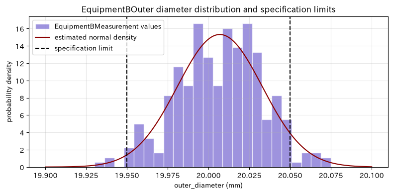
Facility B has an average above the standard center, so there is variation, so attention must be paid to the upper limit side of the non-standard. Although the in-standard rate and observation rate based on the estimated normal distribution are close, normality is not automatically guaranteed. In mass production data, we check time series drift, lot differences, mixing distributions, and outliers, confirm stability, and then extrapolate to future standard rates. Measures that return the mean to the center and those that reduce the standard deviation are managed separately.

---

No.053: Exponential Distribution

Meaning in Practice

During periods when contingent failures occur at a certain rate, the wait time until the next failure can be approximated by an exponential distribution. It can be used to estimate the frequency of maintenance personnel calls and the probability of operating without breakdowns for a certain period.

Approach to Analysis and Modeling

The exponential distribution of failure rate $\lambda>0$ is

$$f(t)=\lambda e^{-\lambda t},\quad S(t)=P(T>t)=e^{-\lambda t},\quad E[T]=\frac{1}{\lambda}$$

That’s right. An important trait is amnesia.

$$P(T>s+t\mid T>s)=P(T>t)$$

That’s right. This does not mean that ‘equipment that has been running for a long time is more prone to breakage.’ If there is wear, consider No.060 Weibull distribution, etc.

Check with Python

intervals = failure_df["interval_between_accidental_failures_h"]
mean_hat = intervals.mean()
lambda_hat = 1 / mean_hat
s, t = 72, 48
conditional_emp = (intervals > s + t).sum() / (intervals > s).sum()

display(pd.DataFrame({
    "mean_time_between_failures_h": [mean_hat],
    "estimated_failure_rate_1/h": [lambda_hat],
    "P(T>48)theory": [np.exp(-lambda_hat * t)],
    "P(T>120|T>72)specimen": [conditional_emp],
}).round(4))

time_grid = np.linspace(0, 400, 500)
fig, ax = plt.subplots(figsize=(8, 4))
ax.hist(intervals, bins=25, density=True, alpha=0.7, color="teal",
        edgecolor="white", label="Interval of failures")
ax.plot(time_grid, stats.expon.pdf(time_grid, scale=mean_hat), color="darkred", label="estimated exponential density")
ax.set_title("Breakdown intervals assuming accidental breakdowns")
ax.set_xlabel("Interval of failures (h)")
ax.set_ylabel("probability density")
ax.grid(alpha=0.3)
ax.legend()
plt.tight_layout()
plt.show()

	mean_time_between_failures_h	estimated_failure_rate_1/h	P(T>48)theory	P(T>120|T>72)specimen
0	101.9568	0.0098	0.6245	0.6351

Reading the results

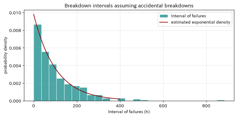
The failure interval is set to the right, allowing estimation of the failure rate from the reciprocal of the sample mean. Sample confirmation with memoryless data is limited in number and does not fully match theoretical values. The core of practice is that adopting the exponential distribution assumes a constant instantaneous failure rate regardless of elapsed time. Failure modes are not mixed; if there is wear, initial failure, or changes in maintenance conditions, sections or modes are separated.

---

No.054: Gamma Distribution

Meaning in Practice

When recovery work consists of multiple stages such as diagnosis, replacement, adjustment, and confirmation, and the required time for each stage fluctuates positively, the total time may be expressed as a gamma distribution. Not only averages, but also the ‘probability of recovery within 4 hours’ and the upper quantile of staff restraining time can be planned.

Approach to Analysis and Modeling

The density of the gamma distribution with shape parameter $k$ and scale parameter $\theta$ is

$$f(x)=\frac{x^{k-1}e^{-x/\theta}}{\Gamma(k)\theta^k},\quad x>0,$$ $$E[X]=k\theta,\qquad \mathrm{Var}(X)=k\theta^2.$$

Adding $k$ independent exponential distributions of the same scale $\theta$ gives the gamma distribution of shape $k$. Here, there are 4 tasks, each averaging 0.8 hours, so the theoretical average is 3.2 hours.

Check with Python

recovery = recovery_df["total_recovery_h"]
k, theta = 4, 0.8
gamma_result = pd.DataFrame({
    "indicator": ["specimen mean(h)", "theoretical mean(h)", "specimen90%position(h)", "theory90%position(h)", "4Theoretical probability within time"],
    "value": [recovery.mean(), k * theta, recovery.quantile(0.9),
          stats.gamma.ppf(0.9, a=k, scale=theta), stats.gamma.cdf(4, a=k, scale=theta)],
})
display(gamma_result.round(4))

grid = np.linspace(0, recovery.max() * 1.05, 500)
fig, ax = plt.subplots(figsize=(8, 4))
ax.hist(recovery, bins=24, density=True, alpha=0.7, color="darkorange",
        edgecolor="white", label="Total recovery time")
ax.plot(grid, stats.gamma.pdf(grid, a=k, scale=theta), color="navy", label="Gamma(4, 0.8)")
ax.axvline(stats.gamma.ppf(0.9, a=k, scale=theta), color="darkred", linestyle="--", label="theory90%position")
ax.set_title("4Total recovery time and gamma distribution of work")
ax.set_xlabel("Total recovery time (h)")
ax.set_ylabel("probability density")
ax.grid(alpha=0.3)
ax.legend()
plt.tight_layout()
plt.show()

	indicator	value
0	specimen mean(h)	3.1670
1	theoretical mean(h)	3.2000
2	specimen90%position(h)	5.3064
3	theory90%position(h)	5.3446
4	4Theoretical probability within time	0.7350

Reading the results

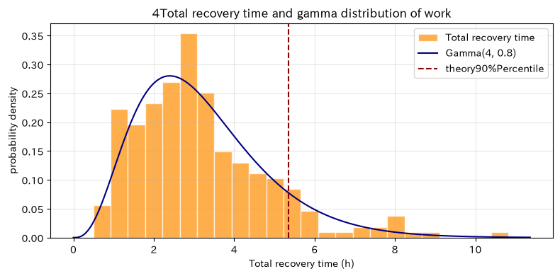
The total recovery time should not be less than zero, and the hem should be held to the right. The sample mean and 90% percentiles are close to theoretical values, so in staffing planning, not only can you use an average of 3.2 hours, but also about 90% of the time to settle. However, setting each task independently with the same scale is a simplification. If part waiting or approval waiting is mixed, wait times are divided into separate KPIs or handled through mixed distribution and simulation.

---

No.055: Beta Distribution

Meaning in Practice

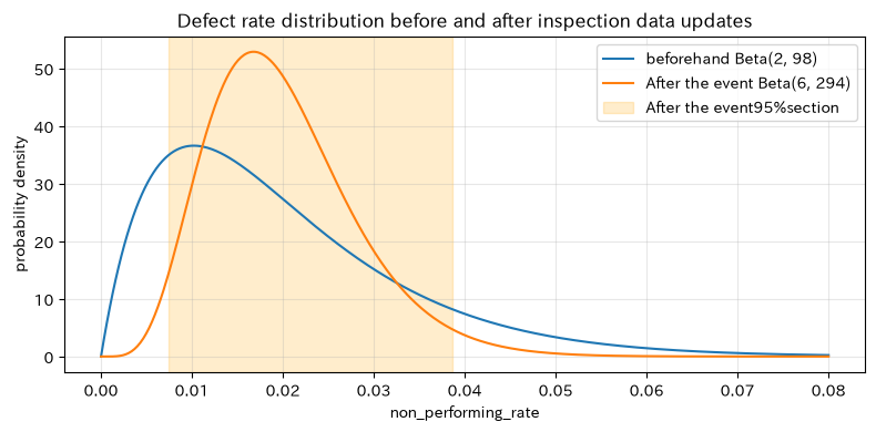
Defect and success rates range from 0 to 1. When data is scarce, such as right after a new product launch, not only is the defect rate 2% scarce, but the uncertainty of the defect rate itself expressed as a beta distribution allows for probabilistic discussions for additional inspections and shipping decisions.

Approach to Analysis and Modeling

The beta distribution of the shape parameter $\alpha,\beta>0$ is

$$f(p)=\frac{p^{\alpha-1}(1-p)^{\beta-1}}{B(\alpha,\beta)},\quad 0<p<1,$$ $$E[P]=\frac{\alpha}{\alpha+\beta},\qquad \mathrm{Var}(P)=\frac{\alpha\beta}{(\alpha+\beta)^2(\alpha+\beta+1)}$$

That’s right. It is also a conjugate prior distribution for binary data; if you observe $d$ defective and $n-d$ good products in prior distribution $\mathrm{Beta}(\alpha_0,\beta_0)$, the posterior distribution becomes $\mathrm{Beta}(\alpha_0+d,\beta_0+n-d)$. Here, we $\mathrm{Beta}(2,98)$ past knowledge and consider 4 out of 200 new tests to be defective.

Check with Python

alpha0, beta0 = 2, 98
n, defects = 200, 4
alpha1, beta1 = alpha0 + defects, beta0 + n - defects
ci_low, ci_high = stats.beta.ppf([0.025, 0.975], alpha1, beta1)

beta_result = pd.DataFrame({
    "distribution": ["beforehand", "After the event"],
    "alpha": [alpha0, alpha1], "beta": [beta0, beta1],
    "average_defect_rate": [alpha0 / (alpha0 + beta0), alpha1 / (alpha1 + beta1)],
})
display(beta_result.round(4))
print(f"After the event95%section: {ci_low:.4%} 〜 {ci_high:.4%}")
print(f"The defect rate3%Exceeding the posterior probability: {stats.beta.sf(0.03, alpha1, beta1):.2%}")

p_grid = np.linspace(0, 0.08, 500)
fig, ax = plt.subplots(figsize=(8, 4))
ax.plot(p_grid, stats.beta.pdf(p_grid, alpha0, beta0), label="beforehand Beta(2, 98)")
ax.plot(p_grid, stats.beta.pdf(p_grid, alpha1, beta1), label="After the event Beta(6, 294)")
ax.axvspan(ci_low, ci_high, color="orange", alpha=0.2, label="After the event95%section")
ax.set_title("Defect rate distribution before and after inspection data updates")
ax.set_xlabel("non_performing_rate")
ax.set_ylabel("probability density")
ax.grid(alpha=0.3)
ax.legend()
plt.tight_layout()
plt.show()

	distribution	alpha	beta	average_defect_rate
0	beforehand	2	98	0.0200
1	After the event	6	294	0.0200

Post-95% interval: 0.7399% to 3.8591%
Post-event probability of defect rate exceeding 3%: 11.38%

Reading the results

The observed defect rate is 4/200 = 2%, but the true defect rate is not fixed at a single point; instead, you can obtain a 95% interval and a “probability of exceeding 3%.” When used for shipment judgment, parties agree on a 3% management standard, loss from false positives, and the basis for pre-distribution with stakeholders. Sensitivity analysis with a different prior distribution is also necessary. Note that the beta distribution represents an unknown rate constrained from 0 to 1, not individual product quality values.

---

No.056: Chi-square Distribution

Meaning in Practice

Standard deviation represents variation in the process, but the sample variance calculated from a small sample also fluctuates. Rather than definitively stating that the standard deviation is 0.02 mm based on just 15 measurements, the chi-square distribution is used to indicate the range within which the population variance can be found.

Approach to Analysis and Modeling

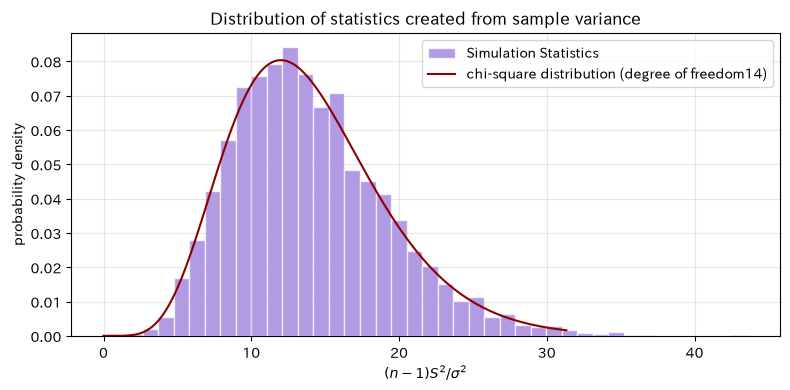
If the population is normally distributed, sample size $n$, unbiased sample variance $S^2$, and population variance $\sigma^2$, then

$$\frac{(n-1)S^2}{\sigma^2}\sim\chi^2_{n-1}.$$

Therefore, the confidence interval of the population variance with confidence coefficient $1-\alpha$ is

$$\left[ \frac{(n-1)S^2}{\chi^2_{1-\alpha/2,n-1}}, \frac{(n-1)S^2}{\chi^2_{\alpha/2,n-1}} \right]$$

That’s right. The sections are not symmetrical; the fewer the samples, the wider they become.

Check with Python

sigma_true = 0.020
n = 15
simulations = 5000
samples = rng.normal(20.0, sigma_true, size=(simulations, n))
sample_vars = samples.var(axis=1, ddof=1)
chi_stats = (n - 1) * sample_vars / sigma_true**2

one_sample = samples[0]
s2 = one_sample.var(ddof=1)
df_chi = n - 1
var_low = df_chi * s2 / stats.chi2.ppf(0.975, df_chi)
var_high = df_chi * s2 / stats.chi2.ppf(0.025, df_chi)

display(pd.DataFrame({
    "specimen_standard_deviation_mm": [np.sqrt(s2)],
    "Population standard deviation95%lower_limit_mm": [np.sqrt(var_low)],
    "Population standard deviation95%upper_mm": [np.sqrt(var_high)],
    "true_standard_deviation_mm": [sigma_true],
}).round(5))

grid = np.linspace(0, stats.chi2.ppf(0.995, df_chi), 500)
fig, ax = plt.subplots(figsize=(8, 4))
ax.hist(chi_stats, bins=40, density=True, alpha=0.7, color="mediumpurple",
        edgecolor="white", label="Simulation Statistics")
ax.plot(grid, stats.chi2.pdf(grid, df_chi), color="darkred", label=f"chi-square distribution (degree of freedom{df_chi})")
ax.set_title("Distribution of statistics created from sample variance")
ax.set_xlabel(r"$(n-1)S^2/\sigma^2$")
ax.set_ylabel("probability density")
ax.grid(alpha=0.3)
ax.legend()
plt.tight_layout()
plt.show()

	specimen_standard_deviation_mm	Population standard deviation95%lower_limit_mm	Population standard deviation95%upper_mm	true_standard_deviation_mm
0	0.0177	0.0130	0.0280	0.0200

Reading the results

The 95% interval of standard deviation obtained from 15 samples is considerably wider than the point estimate. The simulated statistics follow a chi-square distribution with 14 degrees of freedom, allowing you to confirm the meaning of the theoretical formula. This interval depends on the normality and independence of the population. If there is drift, autocorrelation, or outliers in the process, review the process state before using simple sections. Since the reliability of the process capability index also depends on sample size, passing or failing is not determined solely by point estimation.

---

No.057: t-Distribution

Meaning in Practice

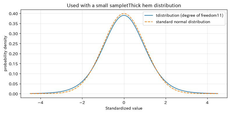
If only 12 measurements are taken during the startup of new equipment, the mother standard deviation is unknown. When the sample mean is standardized by the sample standard deviation, its uncertainty is expressed as a t-distribution with a thicker base than the standard normal distribution. This distribution is designed to avoid overestimating the average value of small data points.

Approach to Analysis and Modeling

For independent samples $X_1,\ldots,X_n$ from a normal population

$$T=\frac{\bar X-\mu}{S/\sqrt{n}}\sim t_{n-1}.$$

The $100(1-\alpha)\%$ confidence interval of the mother mean is

$$\bar X\pm t_{1-\alpha/2,n-1}\frac{S}{\sqrt n}$$

That’s right. As degrees of freedom increase, the t-distribution approaches the standard normal distribution.

Check with Python

startup_sample = quality_df.loc[quality_df["equipment"] == "equipmentB", "outer_diameter_mm"].iloc[:12].to_numpy()
n_t = len(startup_sample)
mean_t = startup_sample.mean()
se_t = startup_sample.std(ddof=1) / np.sqrt(n_t)
t_critical = stats.t.ppf(0.975, df=n_t - 1)
z_critical = stats.norm.ppf(0.975)
t_ci = (mean_t - t_critical * se_t, mean_t + t_critical * se_t)
z_ci = (mean_t - z_critical * se_t, mean_t + z_critical * se_t)

display(pd.DataFrame({
    "Methods": ["tdistribution", "Standard normal distribution (for comparison)"],
    "95%lower_limit_mm": [t_ci[0], z_ci[0]],
    "95%upper_mm": [t_ci[1], z_ci[1]],
    "section_width_mm": [t_ci[1] - t_ci[0], z_ci[1] - z_ci[0]],
}).round(5))

grid = np.linspace(-4.5, 4.5, 500)
fig, ax = plt.subplots(figsize=(8, 4))
ax.plot(grid, stats.t.pdf(grid, df=n_t - 1), label=f"tdistribution (degree of freedom{n_t - 1})")
ax.plot(grid, stats.norm.pdf(grid), linestyle="--", label="standard normal distribution")
ax.set_title("Used with a small sampletThick hem distribution")
ax.set_xlabel("Standardized value")
ax.set_ylabel("probability density")
ax.grid(alpha=0.3)
ax.legend()
plt.tight_layout()
plt.show()

	Methods	95%lower_limit_mm	95%upper_mm	section_width_mm
0	tdistribution	19.9970	20.0302	0.0332
1	Standard normal distribution (for comparison)	19.9988	20.0283	0.0295

Reading the results

Intervals with a t-distribution are wider than those mechanically applied to the standard normal distribution with the same standard error. This reflects the uncertainty of estimating the population standard deviation with a small sample. If the interval is centered on standards or exceeds management tolerances, do not conclude that there is no difference; rather, the current judgment accuracy is insufficient, and consider the value of additional measurements. For a small number of highly non-normal samples, the t-method is also unstable, so confirmation of the measurement process and distribution shape comes first.

---

No.058: F Distribution

Meaning in Practice

Even if the average dimensions of two units are similar, differences in variation can lead to different non-standard risks. The ratio of variance between two groups assuming a normal population follows the F distribution, and differences in variation between facilities can be evaluated using intervals and tests.

Approach to Analysis and Modeling

Let the independent variance of two independent samples $S_1^2,S_2^2$ and the population variance be $\sigma_1^2,\sigma_2^2$,

$$\frac{S_1^2/\sigma_1^2}{S_2^2/\sigma_2^2}\sim F_{n_1-1,n_2-1}.$$

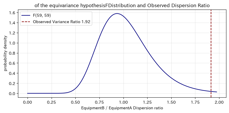
In the null hypothesis that the population variances are equal, $F=S_1^2/S_2^2$ is compared to the F distribution. However, the F test is sensitive to non-normality and outliers. In practice, robust methods such as box beard diagrams, time series, and Levene tests are also employed.

Check with Python

a = quality_df.loc[quality_df["equipment"] == "equipmentA", "outer_diameter_mm"].iloc[:60].to_numpy()
b = quality_df.loc[quality_df["equipment"] == "equipmentB", "outer_diameter_mm"].iloc[:60].to_numpy()
var_a, var_b = a.var(ddof=1), b.var(ddof=1)
f_stat = var_b / var_a
df1, df2 = len(b) - 1, len(a) - 1
p_value = 2 * min(stats.f.cdf(f_stat, df1, df2), stats.f.sf(f_stat, df1, df2))
ratio_low = f_stat / stats.f.ppf(0.975, df1, df2)
ratio_high = f_stat / stats.f.ppf(0.025, df1, df2)

display(pd.DataFrame({
    "equipmentB/ASample variance ratio": [f_stat],
    "Parent dispersion ratio95%lower_limit": [ratio_low],
    "Parent dispersion ratio95%upper": [ratio_high],
    "both sidespvalue": [min(p_value, 1.0)],
}).round(4))

grid = np.linspace(0, stats.f.ppf(0.995, df1, df2), 500)
fig, ax = plt.subplots(figsize=(8, 4))
ax.plot(grid, stats.f.pdf(grid, df1, df2), color="navy", label=f"F({df1}, {df2})")
ax.axvline(f_stat, color="darkred", linestyle="--", label=f"Observed Variance Ratio {f_stat:.2f}")
ax.set_title("of the equivariance hypothesisFDistribution and Observed Dispersion Ratio")
ax.set_xlabel("equipmentB / equipmentA Dispersion ratio")
ax.set_ylabel("probability density")
ax.grid(alpha=0.3)
ax.legend()
plt.tight_layout()
plt.show()

	equipmentB/ASample variance ratio	Parent dispersion ratio95%lower_limit	Parent dispersion ratio95%upper	both sidespvalue
0	1.9165	1.1448	3.2085	0.0136

Reading the results

The variance ratio of equipment B/A is greater than 1, and from the 95% interval and p-value, we can obtain evidence indicating that equipment B has significant variation in this setting. However, statistical differences alone do not determine the priority of improvement investments. We evaluate how much loss would result when the variance is converted into the number of non-standard items, rework time, and customer impact. We also check whether the product configurations and measuring instruments for each equipment are the same, and check whether a single outlier can change the conclusion.

---

No.059: Log-normal Distribution

Meaning in Practice

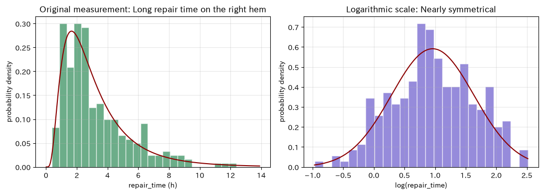
Repair time rarely drops below zero, and in many cases, it can be completed in a short time, but diagnostic difficulties and parts procurement can take a very long time. The amount of multiple multiplier factors that accumulate may approach a normal distribution when taken logarithmically, but may become log-normal on the original scale.

Approach to Analysis and Modeling

When $Y=\log X$ follows $N(\mu,\sigma^2)$, $X$ follows a lognormal distribution,

$$f(x)=\frac{1}{x\sigma\sqrt{2\pi}} \exp\left\{-\frac{(\log x-\mu)^2}{2\sigma^2}\right\},\quad x>0,$$ $$\mathrm{median}(X)=e^\mu,\qquad E[X]=e^{\mu+\sigma^2/2}$$

That’s right. Because the right hem is long, the average is larger than the median. KPIs are divided by purpose, such as the median for typical time and average or upper quantiles for personnel and downtime losses.

Check with Python

repair = repair_df["repair_time_h"]
log_repair = np.log(repair)
mu_log, sigma_log = log_repair.mean(), log_repair.std(ddof=1)
mean_model = np.exp(mu_log + sigma_log**2 / 2)
median_model = np.exp(mu_log)
p95_model = stats.lognorm.ppf(0.95, s=sigma_log, scale=np.exp(mu_log))

display(pd.DataFrame({
    "indicator": ["specimen mean", "Median sample", "Model Mean", "Model Median", "Model95%position"],
    "repair_time_h": [repair.mean(), repair.median(), mean_model, median_model, p95_model],
}).round(3))

grid = np.linspace(0.01, repair.quantile(0.995) * 1.2, 500)
fig, axes = plt.subplots(1, 2, figsize=(11, 4))
axes[0].hist(repair, bins=25, density=True, alpha=0.7, color="seagreen", edgecolor="white")
axes[0].plot(grid, stats.lognorm.pdf(grid, s=sigma_log, scale=np.exp(mu_log)), color="darkred")
axes[0].set_title("Original measurement: Long repair time on the right hem")
axes[0].set_xlabel("repair_time (h)")
axes[0].set_ylabel("probability density")
axes[0].grid(alpha=0.3)
axes[1].hist(log_repair, bins=25, density=True, alpha=0.7, color="slateblue", edgecolor="white")
log_grid = np.linspace(log_repair.min(), log_repair.max(), 500)
axes[1].plot(log_grid, stats.norm.pdf(log_grid, mu_log, sigma_log), color="darkred")
axes[1].set_title("Logarithmic scale: Nearly symmetrical")
axes[1].set_xlabel("log(repair_time)")
axes[1].set_ylabel("probability density")
axes[1].grid(alpha=0.3)
plt.tight_layout()
plt.show()

	indicator	repair_time_h
0	specimen mean	3.2540
1	Median sample	2.4820
2	Model Mean	3.2810
3	Model Median	2.6130
4	Model95%position	7.9280

Reading the results

On the original scale, the average exceeds the median, with a few long-term repairs pushing up the average downtime. If you estimate personnel and losses based only on the median, you will underestimate the deal for a long time, and if you only use the maximum value, you will be swayed by chance. It is effective to report the mean, median, and 90% and 95% percentiles by role. If another pile occurs while waiting for parts, do not push it into a single log-normal distribution; instead, separate the “actual working time” from the “waiting time.”

---

No.060: Weibull Distribution

Meaning in Practice

The lifespan of bearings, seals, tools, and other components changes over time as their likelihood of failure changes. The Weibull distribution can represent initial failures, accidental failures, and wear failures based on the shape parameter, and is widely used for considering preventive replacement cycles and warranty periods.

Approach to Analysis and Modeling

The Weibull distribution with shape parameter $k$ and scale parameter $\lambda$ is

$$f(t)=\frac{k}{\lambda}\left(\frac{t}{\lambda}\right)^{k-1} \exp\left\{-\left(\frac{t}{\lambda}\right)^k\right\},$$ $$S(t)=\exp\left\{-\left(\frac{t}{\lambda}\right)^k\right\},\qquad h(t)=\frac{k}{\lambda}\left(\frac{t}{\lambda}\right)^{k-1}.$$

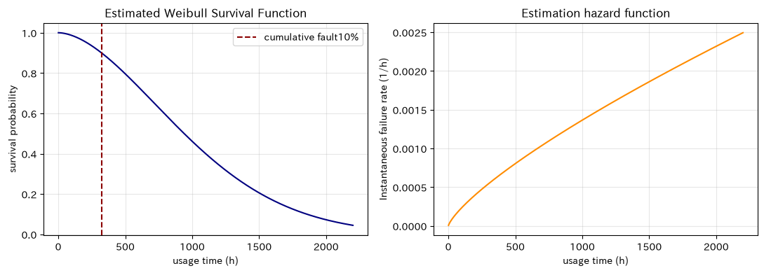
$k<1$ Failure rates decrease,$k=1$ is constant,$k>1$ indicates an increase in failure rates. scale $\lambda$ The survival rate is $e^{-1}\approx36.8\%$ It is not the average lifespan itself.

Check with Python

life = life_df["component_lifespan_h"]
# For fictitious data with no cut-off, the parameter is estimated at fixed position 0
shape_hat, loc_hat, scale_hat = stats.weibull_min.fit(life, floc=0)
replace_at_10pct_failure = scale_hat * (-np.log(0.90)) ** (1 / shape_hat)
median_life = stats.weibull_min.ppf(0.5, shape_hat, scale=scale_hat)

display(pd.DataFrame({
    "presumed shapek": [shape_hat], "estimated_scale_lambda_h": [scale_hat],
    "estimated_median_h": [median_life],
    "cumulative fault10%the_time_h": [replace_at_10pct_failure],
}).round(2))

time_grid = np.linspace(1, 2200, 500)
survival = stats.weibull_min.sf(time_grid, shape_hat, scale=scale_hat)
hazard = (shape_hat / scale_hat) * (time_grid / scale_hat) ** (shape_hat - 1)

fig, axes = plt.subplots(1, 2, figsize=(11, 4))
axes[0].plot(time_grid, survival, color="navy")
axes[0].axvline(replace_at_10pct_failure, color="darkred", linestyle="--", label="cumulative fault10%")
axes[0].set_title("Estimated Weibull Survival Function")
axes[0].set_xlabel("usage_time (h)")
axes[0].set_ylabel("survival probability")
axes[0].grid(alpha=0.3)
axes[0].legend()
axes[1].plot(time_grid, hazard, color="darkorange")
axes[1].set_title("Estimation hazard function")
axes[1].set_xlabel("usage_time (h)")
axes[1].set_ylabel("Instantaneous failure rate (1/h)")
axes[1].grid(alpha=0.3)
plt.tight_layout()
plt.show()

	presumed shapek	estimated scalelambda_h	estimated_median_h	cumulative fault10%the_time_h
0	1.7600	1,156.4200	939.4800	322.9300

Reading the results

The estimated shape parameter is greater than 1, indicating a wear type where the instantaneous failure rate increases with usage time. If the service level is to keep cumulative failures within 10%, the time required to meet those conditions becomes a candidate for the replacement cycle. However, instead of simply adopting the points calculated here, optimization is based on the total cost, including planned downtime cost, sudden downtime cost, initial failure after replacement, inventory, and replacement work capacity. Since most of the practical lifespan data are not broken during the observation period, simply applying the distribution to defective products shortens the lifespan.

Practical Implications Seen Through Target Exercise

Through No.051 to No.060, continuous distribution can be organized into the following four roles.

1. Designing Observations: Uniformly distributed to ensure fair selection of testing locations and times
2. Expressing a phenomenon: Normal, exponential, gamma, lognormal, and Weibull distributions are aligned with the generation mechanism
3. Expressing the uncertainty of unknown quantities: Deals with defect rate using beta distribution, variance with chi-square distribution, and average of small samples using t-distribution
4. Compare the processes: Evaluate the variance ratio using the F distribution and convert the difference into out-of-standard or loss-based

The order of distribution selection is not enough to simply “look for curves similar to the histogram.” First, check the scope of target quantity, generation process, independence, time changes, termination, and the edges of the decision to prioritize.

subject of judgment	Why the center alone is not enough	Indicators to be noted alongside
dimensional quality	Even when the average is the center, there are variations that lead to out-of-standard results.	Standard deviation, in-specification rate, time series
Recovery Plan	Due to the right hem, over-average is frequent.	Median, around 90% and 95%
New Process Evaluation	Estimates can fluctuate greatly in small sample sizes	Confidence intervals, additional measurements
preventive maintenance	Failure rates vary with usage time	Survival Probability, Hazards, Total Cost

What is necessary for practical implementation

1. Fix the analysis unit and data definitions

Define equipment ID, product, material lot, measuring instrument, failure mode, shutdown start and recovery times, and whether it is a planned or sudden stop. Standardize the start and end conditions for KPIs, such as including parts waiting times in repair times.

2. Check the stratification and time series first

When different equipment, products, and failure modes are mixed, it becomes less like a single distribution. Process stability is checked using control charts and time series to evaluate the distribution after stratification. It is also important not to treat correlated continuous measurements as independent samples.

3. Examine not just fit but also the hem of your decision

Using Q-Q plots, cumulative experience distributions, residuals, AIC, and more, we check errors near the specification limits and the 95th percentile. Even if the fit to the center is good, if the right hem that determines the stop loss does not fit, it will not be suitable for the intended purpose.

4. Manage cancellations, missed measurements, and selection bias

In lifetime analysis, undamaged products are retained as cut-offs. Recording processes such as only major failures, missing short-term stoppages, or changing inspection locations based on on-site judgment are also digitized.

5. Connecting probabilities to costs and operational rules

Convert non-standard rates, downtime probabilities, and replacement cycles into disposal costs, delivery delays, spare parts, maintenance personnel, and customer impact. Regularly update the model and determine the responsible person, frequency, and criteria to monitor deviations between forecast probability and actual performance.

Conclusion

• Uniform distribution can be used for randomization of test locations, while normal distribution can be used for approximation of stable dimensional variation
• The exponential distribution represents a constant failure rate, while the gamma distribution represents the sum of multiple positive latency times
• The beta distribution represents the uncertainty of the 0–1 rate and can be updated by test results
• Chi-square, t-distribution, and F-distribution support the inference of variance and the mean and proportion of variance for small samples
• The log-normal distribution is suited for long repair times on the right side, while the Weibull distribution is suited for failure rates that change over time
• Distribution is selected based on the mechanism of occurrence and decision-making objectives, and the fit is checked by stratification, time series, cutoffs, and hem

The value of using continuous distribution in practice lies in not reducing field variability to a single average but converting it into “which events occur, by when, and with what probability.”

Consultations for Corporations

At Surikoubo, we provide the following support targeting quality, production, and maintenance data from manufacturing industries.

• Process capability, non-standard rate, and visualization of inspection design
• Distribution Analysis of Breakdown, Repair, and Lifespan Data and Preventive Maintenance Design
• Support for Statistical Models, Simulations, and KPI Design
• Python and statistical training tailored to actual manufacturing data
• Establishing a system to embed analysis results in on-site operations and management meetings

📩 Contact Us: surikobo.co.jp/contact
Please feel free to consult us first.