From Sampling Inspection to Process Estimation: Judging Manufacturing Conditions with Limited Data

Using precision component processes where it is impossible to measure all quantities, we consistently address the concept of estimating populations from samples, covering the nature of estimation quantities, the most likelihood method, information content, limits of estimation accuracy, and separation of mixing processes. By back-and-forth between formulas and Python simulations, manufacturers connect “how many points should be measured,” “how reliable are those estimates?”, and “how to interpret the mixed data” to manufacturing decision-making.

[!NOTE] This material is a notebook previously used by Surikoubo (or personally by the representative, Kazuyama), and has been reconstructed, edited, and published with the company’s permission. All data listed is fictional and has no relation whatsoever to real companies, factories, or figures.

Introduction: Practical Challenges in Manufacturing Covered in This Article

In mass production, precisely measuring the dimensions of all manufactured quantities may not be realistic due to measurement time, equipment capacity, and cost. Therefore, we extract a portion from each lot to estimate average dimensions, variation, and nonconformity rates, and determine shipment, condition correction, and additional inspection.

However, the sample values change each time you take them. Just because the sample mean is close to the standard center does not necessarily mean the entire process is stable; the nature of the estimation varies depending on the method of calculating sample variance and sample size. In this article, we will treat not only the estimates themselves but also Bias and variation, information content, and theoretical accuracy limits as a basis for judgment.

Common situations on site

• The tradition of 10 points per lot continues, but the score is not determined based on the required estimation accuracy
• The monthly average is confirmed, but the population, sample range, period, and sampling method are ambiguous.
• Whether to use $n$ or $n-1$ in sample variance varies depending on the person in charge or the tool
• While the estimates are reported in detail to the nearest decimal places, the standard error is not also included
• Measurements from multiple facilities and conditions are mixed, and the average and variance are calculated as a single distribution

In such a state, even if the calculations are correct, decisions can be made incorrectly. First, you need to define the estimation target and align the extraction design with the estimation method.

Why is this issue so difficult to judge?

The true mean or variance of the population is usually not observable. Only a finite number of extracted data can be observed. Even when extracting samples from the same process, the sample mean varies each time, and the smaller the sample size, the larger the swing. Also, if the composition ratios of equipment, shifts, and material lots are skewed, not only will random errors occur, but systematic biases will also occur.

Therefore, “just a few estimates” is not enough. Manage the target population, sampling method, estimation, standard error, and model assumptions as a single set to determine whether the uncertainty of the estimate is small enough to account for shipment losses and adjustment costs.

Overview of Exercise covered this time

No.	Theme	Questions in the Manufacturing Industry	Main Confirmation Details
081	Specimen and population	Does the extracted data represent the entire process?	Population, Sample, and Sampling Frame
082	specimen mean	What score should be measured to stabilize the average value?	Sample Distribution and Standard Error
083	sample dispersion	How to calculate process variation	Degree of Freedom & $n-1$ Correction
084	unbiased inferred quantitative	Repeated to check for bias in estimation	Bias comparison
085	consensus estimate	Will increasing data bring us closer to the true value?	MSE and sample size
086	sufficient statistical value	Can you summarize the information needed for estimation?	Binomial Models and Nonconformities
087	Most Likely Estimation Method	What are the conditions that best explain the observational data?	Likelihood and Numerical Optimization
088	Fisher Information Volume	How do the number of measurements and accuracy affect estimation power?	Information Volume and Standard Error
089	Kramer Lao Below	What are the limitations of the accuracy of unbiased estimation?	Lower Bounds & Efficiency
090	EM Algorithm	How to separate the mixed process states	Latent Variables and Iterative Estimation

Preparing the Python environment

It does not rely on external data, using only NumPy, pandas, SciPy, and matplotlib. Fix the seed of the random number generator so that tables and graphs can be reproduced in the same environment. The graph is displayed in English to avoid font differences when converting to Markdown.

%matplotlib inline
import platform

import matplotlib.pyplot as plt
import numpy as np
import pandas as pd
import scipy
from IPython.display import display
from scipy import optimize, stats

SEED = 20260711
rng = np.random.default_rng(SEED)
plt.rcParams["figure.figsize"] = (8, 4.5)
plt.rcParams["axes.axisbelow"] = True

print(f"Python      : {platform.python_version()}")
print(f"NumPy       : {np.__version__}")
print(f"pandas      : {pd.__version__}")
print(f"SciPy       : {scipy.__version__}")

Python      : 3.13.1
NumPy       : 2.5.1
pandas      : 3.0.3
SciPy       : 1.18.0

Creation of Fictional Data

Generate 24,000 virtual data for one month by producing precision shafts in two machines (M1, M2) in three shifts. The target is diameter, with a target value of 10,000 mm and a standard of 9,980–10,020 mm. Small mean differences are assigned for each equipment and shift, and stratified sample samples are created from all data.

From then on, all data will be used as a “known finite population” for explanation. In practice, the true population value is unknown, so estimates are made from samples. Additionally, for No.090, mixing measurement data with missing equipment labels is generated separately.

n_population = 24_000
machines = rng.choice(["M1", "M2"], size=n_population, p=[0.58, 0.42])
shifts = rng.choice(["Day", "Evening", "Night"], size=n_population, p=[0.45, 0.35, 0.20])
machine_offset = pd.Series(machines).map({"M1": -0.0015, "M2": 0.0025}).to_numpy()
shift_offset = pd.Series(shifts).map({"Day": 0.0000, "Evening": 0.0008, "Night": -0.0007}).to_numpy()
sigma = np.where(machines == "M1", 0.0060, 0.0075)
diameter = 10.000 + machine_offset + shift_offset + rng.normal(0, sigma)

population_df = pd.DataFrame({
    "unit_id": np.arange(1, n_population + 1),
    "machine": machines,
    "shift": shifts,
    "diameter_mm": diameter,
})
population_df["nonconforming"] = ~population_df["diameter_mm"].between(9.980, 10.020)

# Stratified samples extracted from 80 specimens from each × shift
sample_df = (
    population_df.groupby(["machine", "shift"], group_keys=False)
    .sample(n=80, random_state=SEED)
    .sort_values("unit_id")
    .reset_index(drop=True)
)

# Two-state mixed data with missing labels (No.090)
n_mixed = 700
hidden_state = rng.choice([0, 1], n_mixed, p=[0.64, 0.36])
mixed_values = rng.normal(
    np.where(hidden_state == 0, 9.990, 10.014),
    np.where(hidden_state == 0, 0.0050, 0.0065),
)

display(population_df.head())
display(pd.DataFrame({
    "dataset": ["finite population", "stratified specimen", "Unlabeled mixed data"],
    "rows": [len(population_df), len(sample_df), len(mixed_values)],
}))

	unit_id	machine	shift	diameter_mm	nonconforming
0	1	M1	Night	9.998475	False
1	2	M2	Day	10.015734	False
2	3	M1	Night	9.993877	False
3	4	M2	Night	10.001658	False
4	5	M2	Day	9.999186	False

	dataset	rows
0	finite population	24000
1	stratified specimen	480
2	Unlabeled mixed data	700

---

No.081: Sample and Population — Defining the Subjects of Sampling

Meaning in Practice

The population is “the entire target to be estimated,” and the sample is “the portion actually observed.” For example, whether you use the entire product population for this month as the population or the conceptual population that includes products made under the same conditions in the future will change the scope of the estimate results. If night shifts or specific equipment leak from the sampling slot, even if the measurement score is high, representativeness will not be achieved.

Approach to Analysis and Modeling

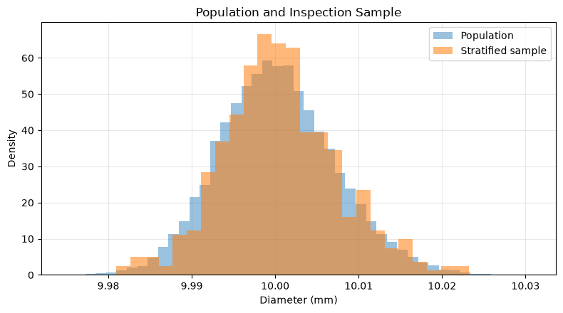
Let the mean of the finite population be $mu_N=N^{-1}\sum_{i=1}^{N}x_i$, and the sample mean be $\bar{x}=n^{-1}\sum_{i=1}^{n}x_i$. In simple random sampling, each individual has an equal chance of extraction. Stratified sampling is done by layer such as equipment or shift, and if the population composition ratio differs from the sample composition ratio, weighting is applied. Here, we compare the distribution and composition of the entire data with the stratified sample.

Check with Python

population_summary = pd.Series({
    "number_of_cases": len(population_df),
    "average_diameter_mm": population_df["diameter_mm"].mean(),
    "standard_deviation_mm": population_df["diameter_mm"].std(ddof=0),
    "nonconformity rate": population_df["nonconforming"].mean(),
})
sample_summary = pd.Series({
    "number_of_cases": len(sample_df),
    "average_diameter_mm": sample_df["diameter_mm"].mean(),
    "standard_deviation_mm": sample_df["diameter_mm"].std(ddof=1),
    "nonconformity rate": sample_df["nonconforming"].mean(),
})
comparison_081 = pd.concat(
    [population_summary.rename("finite population"), sample_summary.rename("stratified specimen")], axis=1
)
display(comparison_081.round(6))

fig, ax = plt.subplots()
ax.hist(population_df["diameter_mm"], bins=45, density=True, alpha=0.45, label="Population")
ax.hist(sample_df["diameter_mm"], bins=25, density=True, alpha=0.55, label="Stratified sample")
ax.set_title("Population and Inspection Sample")
ax.set_xlabel("Diameter (mm)")
ax.set_ylabel("Density")
ax.grid(True, alpha=0.3)
ax.legend()
plt.tight_layout()
plt.show()

	finite population	stratified specimen
number_of_cases	24000.000000	480.00000
average_diameter_mm	10.000264	10.00063
standard_deviation_mm	0.007024	0.00690
nonconformity rate	0.006000	0.00625

Reading the results

The distribution of stratified samples roughly reproduces the center and extent of the population, but the values do not exactly match. This difference is called sampling error. This time, the extraction is evenly divided with 80 stems per layer, so the composition ratio of the population layers differs. When accurately estimating indicators for the entire process, weights are based on population composition ratios, and if equipment comparison is the goal, the level values are reported as-is, thus aligning with the objective. It is important to record the target period, target equipment, exclusion conditions, and extraction methods along with the analysis results.

---

No.082: Sample Mean — Linking Measurement Scores and Average Stability

Meaning in Practice

The sample mean is a basic KPI representing the process center, but the average of the decimal points is influenced by chance. Increasing the number of measurement points stabilizes the average value, but also raises testing costs and assessment time. By using the standard error of the sample mean, you can quantify the trade-off between required accuracy and measurement load.

Approach to Analysis and Modeling

For an independent and identically distributed observation $X_1,\ldots,X_n$, the sample mean is

$$\bar{X}=\frac{1}{n}\sum_{i=1}^{n}X_i,\qquad E[\bar{X}]=\mu,\qquad \mathrm{Var}(\bar{X})=\frac{\sigma^2}{n}$$

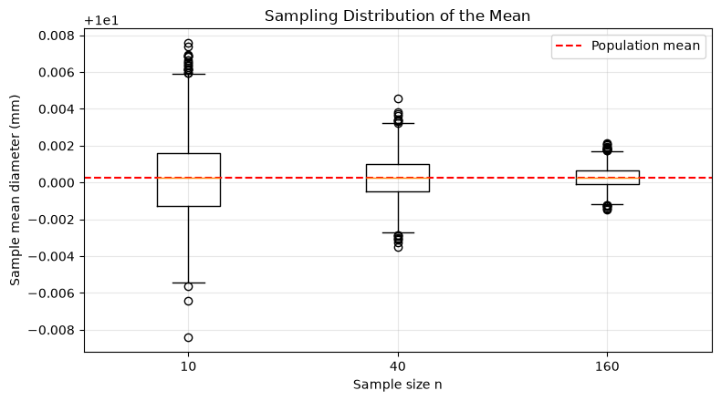
That’s right. Since the standard error decreases at $\sigma/\sqrt{n}$, in principle, four times the data is needed to halve the accuracy. Samples of different sizes are repeatedly extracted from the population to check the distribution of the sample mean.

Check with Python

values = population_df["diameter_mm"].to_numpy()
sample_sizes = [10, 40, 160]
repetitions = 2_000
mean_draws = {
    n: np.array([rng.choice(values, n, replace=False).mean() for _ in range(repetitions)])
    for n in sample_sizes
}
summary_082 = pd.DataFrame([
    {
        "n": n,
        "mean of the sample": draws.mean(),
        "Actual measurement of sample meansSD": draws.std(ddof=1),
        "theorySEsimilar": values.std(ddof=0) / np.sqrt(n),
    }
    for n, draws in mean_draws.items()
])
display(summary_082.round(7))

fig, ax = plt.subplots()
ax.boxplot([mean_draws[n] for n in sample_sizes], tick_labels=[str(n) for n in sample_sizes])
ax.axhline(values.mean(), color="red", linestyle="--", label="Population mean")
ax.set_title("Sampling Distribution of the Mean")
ax.set_xlabel("Sample size n")
ax.set_ylabel("Sample mean diameter (mm)")
ax.grid(True, alpha=0.3)
ax.legend()
plt.tight_layout()
plt.show()

	n	mean of the sample	Actual measurement of sample meansSD	theorySEsimilar
0	10	10.000246	0.002202	0.002221
1	40	10.000261	0.001125	0.001111
2	160	10.000268	0.000566	0.000555

Reading the results

The larger the $n$, the narrower the box of the sample mean, and the measured standard deviation approaches the theoretical standard error. On the other hand, even if the number of measurements is quadrupled, the standard error is only about half. The number of inspection points is not conventional; it is designed using acceptable estimation errors, process standard deviations, measurement costs, and loss of judgment. If there is autocorrelation in continuous production, independence is lost, and the amount of effective information is smaller than in simple formulas.

---

No.083: Sample Variance — Estimating Process Variation Along with Degrees of Freedom

Meaning in Practice

Even if the average is centered around the standard, if there is significant variation, the number of non-standard individuals will increase. Underestimating the variance underlying process capability and control limits leads to an optimistic view of quality risks. Especially in small specimens, the difference between denominating $n$ or $n-1$ cannot be ignored.

Approach to Analysis and Modeling

Since the population mean is also estimated from the sample, there are only $n-1$ pieces of independent information for deviation $X_i-\bar{X}$. Unbiased sample variance is

$$S^2=\frac{1}{n-1}\sum_{i=1}^{n}(X_i-\bar{X})^2$$

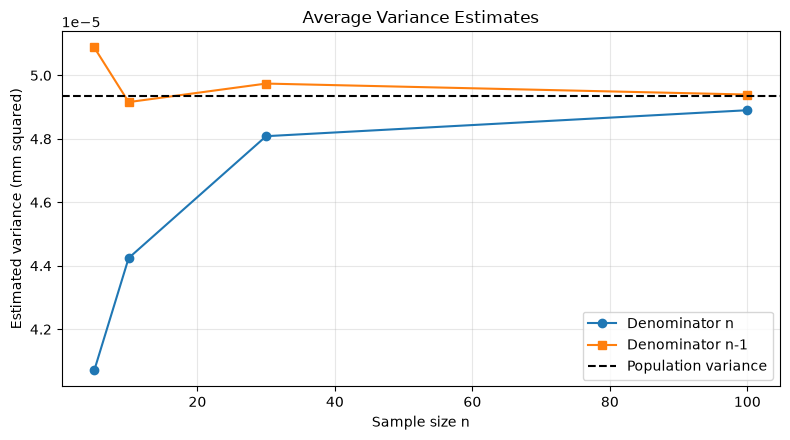
If the variance is finite in an independent and identical distribution, then $E[S^2]=\sigma^2$ is . The variance of the denominator $n$ is the most likely estimate of the normal distribution, but it is generally smaller in finite samples.

Check with Python

true_variance = values.var(ddof=0)
variance_rows = []
for n in [5, 10, 30, 100]:
    draws = rng.choice(values, size=(4_000, n), replace=True)
    variance_rows.append({
        "n": n,
        "denominatornAverage": draws.var(axis=1, ddof=0).mean(),
        "denominatorn-1Average": draws.var(axis=1, ddof=1).mean(),
        "mother dispersion": true_variance,
    })
summary_083 = pd.DataFrame(variance_rows)
display(summary_083.round(9))

fig, ax = plt.subplots()
ax.plot(summary_083["n"], summary_083["denominatornAverage"], "o-", label="Denominator n")
ax.plot(summary_083["n"], summary_083["denominatorn-1Average"], "s-", label="Denominator n-1")
ax.axhline(true_variance, color="black", linestyle="--", label="Population variance")
ax.set_title("Average Variance Estimates")
ax.set_xlabel("Sample size n")
ax.set_ylabel("Estimated variance (mm squared)")
ax.grid(True, alpha=0.3)
ax.legend()
plt.tight_layout()
plt.show()

	n	denominatornAverage	denominatorn-1Average	mother dispersion
0	5	0.000041	0.000051	0.000049
1	10	0.000044	0.000049	0.000049
2	30	0.000048	0.000050	0.000049
3	100	0.000049	0.000049	0.000049

Reading the results

In small samples, the estimated denominator $n$ systematically falls below the population variance, and $n-1$ correction removes this bias. However, being unbiased does not guarantee that a single estimate is close to the true value. Because $n=5$ sample variance varies greatly between iterations, variation monitoring also checks the number of measurements, rational grouping, and time-series changes. If you specify the ddof settings of the library in the data specification, you can prevent calculation differences between departments.

---

No.084: Unbiased Estimators — Examining Long-Term Estimation Bias

Meaning in Practice

If estimation rules slightly underestimate process variation each month, in the long run, inspection standards and capability assessments will shift toward optimism. Unbiasedness is the property where, when sampling is repeated under the same conditions, the mean of the estimate matches the true value.

Approach to Analysis and Modeling

The estimator $\hat{\theta}$ of parameter $\theta$

$E[\hat{\theta}]=\theta$

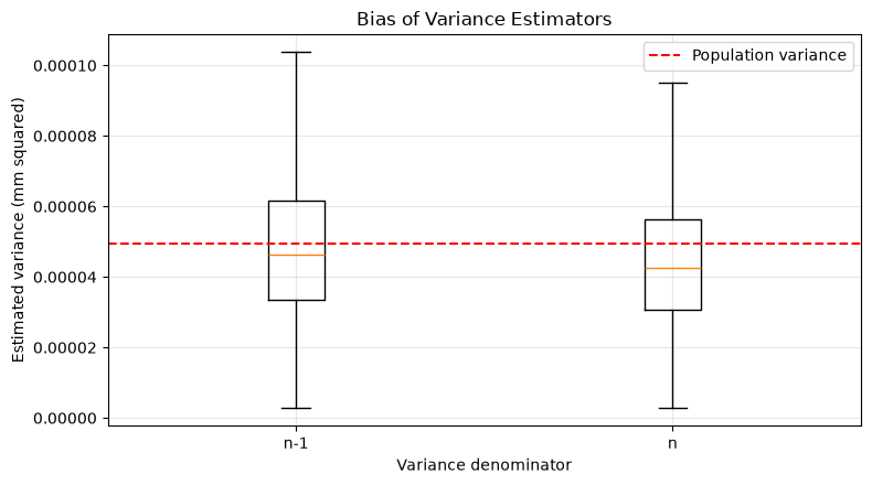
It is called unbiased when the condition is met. The bias is $\mathrm{Bias}(\hat{\theta})=E[\hat{\theta}]-\theta$. The sample variance, which divides the sample mean by $n-1$, is unbiased, but the estimation of variance with denominator $n$ has a $-\sigma^2/n$ bias. Compare three estimation rules in simulation.

Check with Python

n = 12
draws = rng.choice(values, size=(8_000, n), replace=True)
estimators = pd.DataFrame({
    "Estimated Subject": ["mother mean", "mother dispersion", "mother dispersion"],
    "estimated quantity": ["specimen mean", "denominatorn-1sample variance", "denominatornsample variance"],
    "True value": [values.mean(), true_variance, true_variance],
    "Approximate expected value of estimates": [
        draws.mean(axis=1).mean(),
        draws.var(axis=1, ddof=1).mean(),
        draws.var(axis=1, ddof=0).mean(),
    ],
})
estimators["Bias"] = estimators["Approximate expected value of estimates"] - estimators["True value"]
display(estimators.round(9))

variance_estimates = [draws.var(axis=1, ddof=1), draws.var(axis=1, ddof=0)]
fig, ax = plt.subplots()
ax.boxplot(variance_estimates, tick_labels=["n-1", "n"], showfliers=False)
ax.axhline(true_variance, color="red", linestyle="--", label="Population variance")
ax.set_title("Bias of Variance Estimators")
ax.set_xlabel("Variance denominator")
ax.set_ylabel("Estimated variance (mm squared)")
ax.grid(True, alpha=0.3)
ax.legend()
plt.tight_layout()
plt.show()

	Estimated Subject	estimated quantity	True value	Approximate expected value of estimates	Bias
0	mother mean	specimen mean	10.000264	10.000287	2.290500e-05
1	mother dispersion	denominatorn-1sample variance	0.000049	0.000049	-7.500000e-08
2	mother dispersion	denominatornsample variance	0.000049	0.000045	-4.181000e-06

Reading the results

The sample mean and $n-1$ of sample variance match true values within the range of simulation error, and the estimated value of denominator $n$ has a negative bias as expected. However, in practice, estimates are not chosen based solely on imbias. Since allowing some bias can significantly reduce the fluctuation in estimates, we also compare mean squared error, loss in case of anomalies, and explainability. Also, if the sampling itself is biased, even an estimate that is mathematically unbiased will not be unbiased for the target population.

---

No.085: Matched Estimator — Checking if data increases lead to closer to the true value

Meaning in Practice

Even if you increase the amount of data by introducing sensors or automatic measuring machines, if the estimation method is not appropriate, you may not always approach the true value. Consistency is the property where the estimate probabilistically approaches the true parameter when the sample size is increased. It is also a condition that supports the value of long-term data accumulation.

Approach to Analysis and Modeling

For any $\varepsilon>0$

$$P(|\hat{\theta}_n-\theta|>\varepsilon)\to 0\quad(n\to\infty)$$

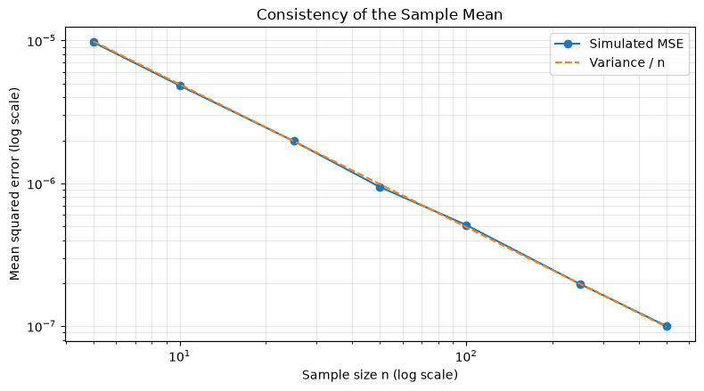
Then $\hat{\theta}_n$ is a consistent estimate. In sample means, consistency is achieved by the law of large numbers, and the mean squared error decreases by about $\sigma^2/n$ if independent and identically distributed. Measurement of error and tolerance rate for data volume is measured.

Check with Python

mu = values.mean()
epsilon = 0.001  # 1 micrometer
consistency_rows = []
for n in [5, 10, 25, 50, 100, 250, 500]:
    sample_means = rng.choice(values, size=(3_000, n), replace=True).mean(axis=1)
    consistency_rows.append({
        "n": n,
        "MSE": np.mean((sample_means - mu) ** 2),
        "absolute error1μmsuper percentage": np.mean(np.abs(sample_means - mu) > epsilon),
    })
summary_085 = pd.DataFrame(consistency_rows)
display(summary_085.round(8))

fig, ax = plt.subplots()
ax.loglog(summary_085["n"], summary_085["MSE"], "o-", label="Simulated MSE")
ax.loglog(summary_085["n"], true_variance / summary_085["n"], "--", label="Variance / n")
ax.set_title("Consistency of the Sample Mean")
ax.set_xlabel("Sample size n (log scale)")
ax.set_ylabel("Mean squared error (log scale)")
ax.grid(True, which="both", alpha=0.3)
ax.legend()
plt.tight_layout()
plt.show()

	n	MSE	absolute error1μmsuper percentage
0	5	9.720000e-06	0.757000
1	10	4.840000e-06	0.655667
2	25	1.970000e-06	0.468333
3	50	9.400000e-07	0.301000
4	100	5.100000e-07	0.157667
5	250	2.000000e-07	0.023333
6	500	1.000000e-07	0.001000

Reading the results

As the sample size increases, the margin of error between MSE and over 1 μm decreases, confirming consistency of sample means. However, for correlation data measured frequently from the same equipment conditions, measurements including calibration deviations, and future process changes, simply increasing the number of cases will not eliminate errors. Consistency is a property under model assumptions. Representativeness across equipment, materials, and periods, as well as measurement bias and drift, are managed separately.

---

No.086: Sufficient Statistics — Aggregating Estimated Information into Nonconformities

Meaning in Practice

There is no need to display all raw test results in meeting materials. If information about the estimated target can be summarized without loss, monitoring, communication, storage, and explanation can be made concise. However, “sufficient” refers to properties related to specific probabilistic models and parameters, and does not mean that the chronological sequence or equipment information necessary for cause analysis is no longer necessary.

Approach to Analysis and Modeling

In the Bernoulli model, where each test independently has a probability of $p$ nonconformity, the likelihood of a total number of nonconformities $T=\sum_i X_i$ out of $n$ cases is

$$L(p\mid\boldsymbol{x})=p^T(1-p)^{n-T}$$

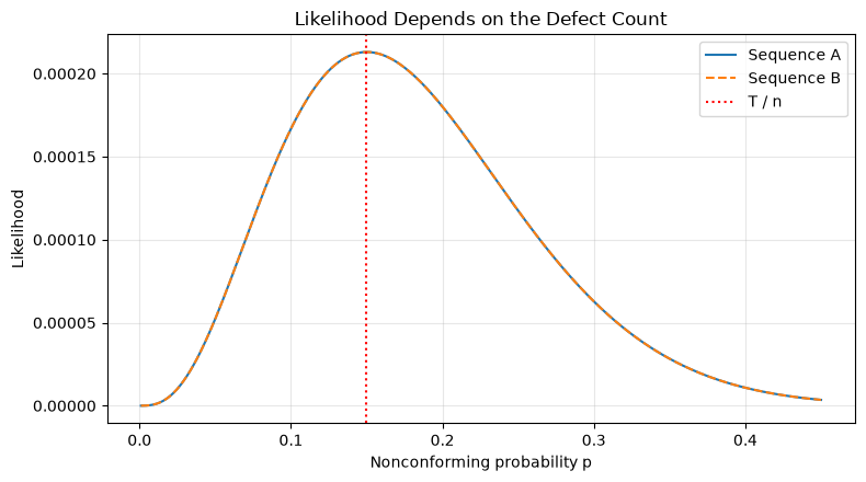
That’s right. Since likelihood depends only on $(n,T)$ rather than the order of the lives, the factorization theorem states that $T$ is a sufficient statistic for $p$. Compare the likelihood of two lines with the same number of cases and the same number of nonconformities, but with a different order of order.

Check with Python

sequence_a = np.array([1, 0, 0, 0, 1, 0, 0, 0, 0, 1, 0, 0, 0, 0, 0, 0, 0, 0, 0, 0])
sequence_b = np.array([0, 0, 1, 0, 0, 0, 0, 1, 0, 0, 0, 0, 0, 0, 0, 0, 0, 0, 1, 0])
p_grid = np.linspace(0.001, 0.45, 400)

def bernoulli_likelihood(sequence, p):
    total = sequence.sum()
    return p ** total * (1 - p) ** (len(sequence) - total)

lik_a = bernoulli_likelihood(sequence_a, p_grid)
lik_b = bernoulli_likelihood(sequence_b, p_grid)
display(pd.DataFrame({
    "series": ["A", "B"],
    "number_of_inspectionsn": [len(sequence_a), len(sequence_b)],
    "non_conforming_numberT": [sequence_a.sum(), sequence_b.sum()],
    "Most Misfit RateT/n": [sequence_a.mean(), sequence_b.mean()],
    "Maximum difference in likelihood curve": [np.max(np.abs(lik_a - lik_b)), np.max(np.abs(lik_a - lik_b))],
}))

fig, ax = plt.subplots()
ax.plot(p_grid, lik_a, label="Sequence A")
ax.plot(p_grid, lik_b, "--", label="Sequence B")
ax.axvline(sequence_a.mean(), color="red", linestyle=":", label="T / n")
ax.set_title("Likelihood Depends on the Defect Count")
ax.set_xlabel("Nonconforming probability p")
ax.set_ylabel("Likelihood")
ax.grid(True, alpha=0.3)
ax.legend()
plt.tight_layout()
plt.show()

	series	number_of_inspectionsn	non_conforming_numberT	Most Misfit RateT/n	Maximum difference in likelihood curve
0	A	20	3	0.15	0.0
1	B	20	3	0.15	0.0

Reading the results

Even if the two series have different sequences, the $(n,T)=(20,3)$ is the same, so the likelihood curves for $p$ overlap completely. If you only estimate the nonconformance rate, you can aggregate information into the number of inspections and nonconformity counts. On the other hand, whether three cases occurred consecutively or concentrated on specific equipment or materials is important for identifying the cause. We retain sufficient statistics for aggregated KPIs and raw data for traceability by purpose, and also monitor assumptions of model independence and identical probabilities.

---

No.087: Maximum Likelihood Estimation Method — Finding the Process Conditions That Most Explain the Observed Dimensions

Meaning in Practice

Consistently calculating process means and standard deviations from data is fundamental for capability assessment, condition correction, and anomaly detection. The Most Likelihood estimation method selects the parameters where the observed data is most likely to occur. This is an estimation principle common to many statistical and machine learning models.

Approach to Analysis and Modeling

If dimension $x_i$ independently follows a normal distribution $N(\mu,\sigma^2)$, then the log-likelihood is

$$\ell(\mu,\sigma)=-n\log\sigma-\frac{n}{2}\log(2\pi) -\frac{1}{2\sigma^2}\sum_{i=1}^{n}(x_i-\mu)^2$$

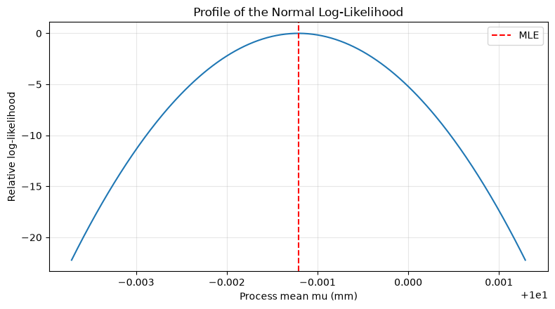
That’s right. Maximizing it yields $\hat{\mu}=\bar{x}$ and $\hat{\sigma}^2=n^{-1}\sum_i(x_i-\bar{x})^2$. Compare the analysis solution with the results of numerical optimization.

Check with Python

m1_data = sample_df.loc[sample_df["machine"] == "M1", "diameter_mm"].to_numpy()

def normal_negative_loglik(params, x):
    mu_value, log_sigma = params
    sigma_value = np.exp(log_sigma)
    return -np.sum(stats.norm.logpdf(x, loc=mu_value, scale=sigma_value))

result = optimize.minimize(
    normal_negative_loglik,
    x0=np.array([m1_data.mean(), np.log(m1_data.std(ddof=1))]),
    args=(m1_data,),
    method="BFGS",
)
mu_mle, sigma_mle = result.x[0], np.exp(result.x[1])
display(pd.DataFrame({
    "method": ["Analytic MLE", "Numerical MLE"],
    "mu": [m1_data.mean(), mu_mle],
    "sigma": [m1_data.std(ddof=0), sigma_mle],
    "converged": [True, result.success],
}).round(8))

mu_grid = np.linspace(mu_mle - 0.0025, mu_mle + 0.0025, 300)
relative_loglik = np.array([
    -normal_negative_loglik((mu_value, np.log(sigma_mle)), m1_data) for mu_value in mu_grid
])
relative_loglik -= relative_loglik.max()
fig, ax = plt.subplots()
ax.plot(mu_grid, relative_loglik)
ax.axvline(mu_mle, color="red", linestyle="--", label="MLE")
ax.set_title("Profile of the Normal Log-Likelihood")
ax.set_xlabel("Process mean mu (mm)")
ax.set_ylabel("Relative log-likelihood")
ax.grid(True, alpha=0.3)
ax.legend()
plt.tight_layout()
plt.show()

	method	mu	sigma	converged
0	Analytic MLE	9.99879	0.005808	True
1	Numerical MLE	9.99879	0.005808	True

Reading the results

If the analytical solution matches the numerical solution, the log-likelihood is maximized by the estimated mean. While most likelihood estimation can be extended to complex models, if assumptions of normality, independence, or single-step are incorrect, the meaning of the resulting value will also change. Also, the maximum likelihood estimator of variance is the denominator $n$, which differs in purpose and nature from the unbiased variance of No.083. It records the estimation method name, likelihood, convergence determination, initial value, and fit diagnosis to distinguish between optimization success and model validity.

---

No.088: Fisher Information Amount — Assessing estimation power based on measurement numbers and accuracy

Meaning in Practice

Even with the same 100 points, the information obtained about the process average differs when measuring stable processes with high-precision instruments versus when measuring variable processes in environments with large measurement errors. The amount of Fisher information indicates how sharply the likelihood changes around unknown parameters, linking the number of tests, measurement accuracy, and estimation accuracy.

Approach to Analysis and Modeling

Score $\partial\ell/\partial\theta$ Expected Square Value of Fisher Information

$$I(\theta)=E\left[\left(\frac{\partial}{\partial\theta}\log f(X;\theta)\right)^2\right]$$

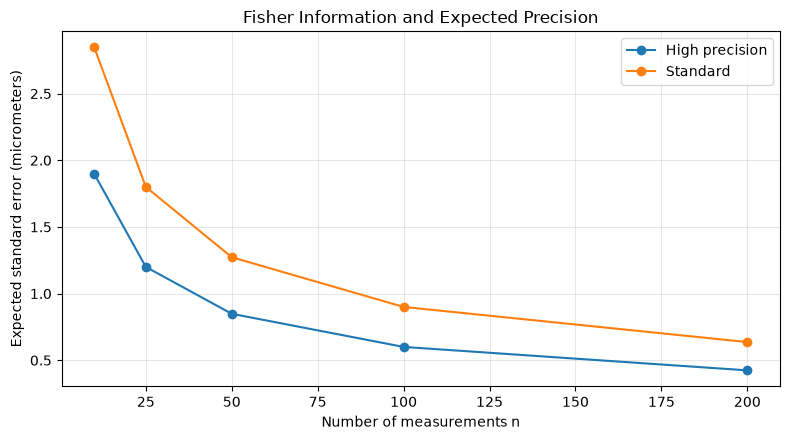
That’s how it is defined. If the variance $\sigma^2$ estimates mean $\mu$ from a known normal distribution, the amount of information from one observation is $1/\sigma^2$, and $I_n(\mu)=n/\sigma^2$ from $n$ observation. The inversesquare root $1/\sqrt{I_n}=\sigma/\sqrt{n}$ of the amount of information serves as a measure of estimation accuracy.

Check with Python

design_rows = []
for measurement_system, sigma_value in [("High precision", 0.006), ("Standard", 0.009)]:
    for n in [10, 25, 50, 100, 200]:
        information = n / sigma_value**2
        design_rows.append({
            "measurement_system": measurement_system,
            "n": n,
            "sigma_mm": sigma_value,
            "Fisher_information": information,
            "expected_SE_mm": 1 / np.sqrt(information),
        })
information_df = pd.DataFrame(design_rows)
display(information_df.round(7))

fig, ax = plt.subplots()
for name, group in information_df.groupby("measurement_system"):
    ax.plot(group["n"], group["expected_SE_mm"] * 1000, "o-", label=name)
ax.set_title("Fisher Information and Expected Precision")
ax.set_xlabel("Number of measurements n")
ax.set_ylabel("Expected standard error (micrometers)")
ax.grid(True, alpha=0.3)
ax.legend()
plt.tight_layout()
plt.show()

	measurement_system	n	sigma_mm	Fisher_information	expected_SE_mm
0	High precision	10	0.006	2.777778e+05	0.001897
1	High precision	25	0.006	6.944444e+05	0.001200
2	High precision	50	0.006	1.388889e+06	0.000848
3	High precision	100	0.006	2.777778e+06	0.000600
4	High precision	200	0.006	5.555556e+06	0.000424
5	Standard	10	0.009	1.234568e+05	0.002846
6	Standard	25	0.009	3.086420e+05	0.001800
7	Standard	50	0.009	6.172840e+05	0.001273
8	Standard	100	0.009	1.234568e+06	0.000900
9	Standard	200	0.009	2.469136e+06	0.000636

Reading the results

The more measurements you take, the lower the expected standard error becomes, but due to the square rule, the marginal effect decreases. Also, high-precision systems with small standard deviations can contain more information even with the same number of measurements. This means that the addition of test points and improvements to the measurement system can be compared using the same accuracy indicator. However, process variations and measurement errors may be mixed in $\sigma$ of the equation. Measurement system variations are separated using tools like Gage R&R and inspection design is selected by considering cost, cycle time, and required accuracy.

---

No.089: Kramer Lao Lower Boundary — Understanding the Accuracy Limits of Unbiased Estimation

Meaning in Practice

Complicating estimation algorithms does not necessarily improve accuracy. Under a given model and data volume, there is a theoretical lower limit for the variance of unbiased estimators. Knowing the lower bound allows you to distinguish between areas where method improvement can be made and areas that need improvement, such as the number of measurements and measurement accuracy.

Approach to Analysis and Modeling

Under regular conditions, the unbiased estimator $\hat{\theta}$ has a Kramer-Rao lower bound

$$\mathrm{Var}(\hat{\theta})\geq\frac{1}{I_n(\theta)}$$

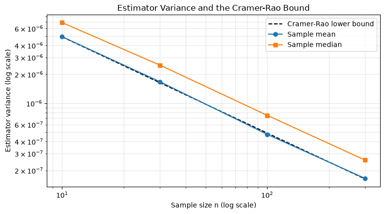
This holds. For the mean of a known normal distribution, the lower bound is $\sigma^2/n$, and the sample mean is an efficient estimate that achieves this lower bound. Compare the variance between the sample mean and the sample median through simulation.

Check with Python

sigma_known = 0.007
crlb_rows = []
for n in [10, 30, 100, 300]:
    normal_draws = rng.normal(10.0, sigma_known, size=(8_000, n))
    mean_estimator = normal_draws.mean(axis=1)
    median_estimator = np.median(normal_draws, axis=1)
    lower_bound = sigma_known**2 / n
    crlb_rows.append({
        "n": n,
        "CRLB": lower_bound,
        "Variance of the sample mean": mean_estimator.var(ddof=1),
        "Median Variance of the Sample": median_estimator.var(ddof=1),
        "average_efficiency_crlb/disperse": lower_bound / mean_estimator.var(ddof=1),
    })
crlb_df = pd.DataFrame(crlb_rows)
display(crlb_df.round(10))

fig, ax = plt.subplots()
ax.loglog(crlb_df["n"], crlb_df["CRLB"], "k--", label="Cramer-Rao lower bound")
ax.loglog(crlb_df["n"], crlb_df["Variance of the sample mean"], "o-", label="Sample mean")
ax.loglog(crlb_df["n"], crlb_df["Median Variance of the Sample"], "s-", label="Sample median")
ax.set_title("Estimator Variance and the Cramer-Rao Bound")
ax.set_xlabel("Sample size n (log scale)")
ax.set_ylabel("Estimator variance (log scale)")
ax.grid(True, which="both", alpha=0.3)
ax.legend()
plt.tight_layout()
plt.show()

	n	CRLB	Variance of the sample mean	Median Variance of the Sample	average_efficiency_CRLB/disperse
0	10	4.900000e-06	4.922100e-06	6.895100e-06	0.995514
1	30	1.633300e-06	1.673900e-06	2.490800e-06	0.975772
2	100	4.900000e-07	4.748000e-07	7.492000e-07	1.031930
3	300	1.633000e-07	1.656000e-07	2.566000e-07	0.986608

Reading the results

The variance of the sample mean almost matches the lower bound, making it efficient for estimating the mean of the normal model. The variance in the median sample is large, and under the assumption of a normal distribution, efficiency is low. On the other hand, in distributions with outliers or heavy hems, the robustness of the median may be advantageous for decision-making. Kramer-Rao lower bounds depend on conditions such as indecentricity, model regularity, and parameter settings, so they are not a universal ranking for every estimate. It is used in light of field distribution and loss functions.

---

No.090: EM Algorithm — Estimating Unlabeled Mixing Processes Iteratively

Meaning in Practice

If records of equipment IDs or setup conditions are missing, measurements from different process states are mixed into a single distribution. Using the overall average alone overlooks the two states at different centers or variations by state. The EM algorithm estimates the parameters of each state while probabilistically supplementing latent labels indicating which state it was generated from.

Approach to Analysis and Modeling

Two-component normal mixing model

$$p(x)=\sum_{k=1}^{2}\pi_k\,\mathcal{N}(x\mid\mu_k,\sigma_k^2)$$

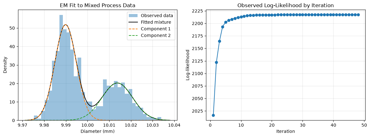
Let’s say so. In Step E, calculate the post-hoc probability (responsibility level) $r_{ik}$ for each observation belonging to component $k$ from the current parameters. In the M Step, the $\pi_k,\mu_k,\sigma_k^2$ is updated with accountability as a weight. Repeat until the increase in log-likelihood becomes sufficiently small.

Check with Python

def gaussian_mixture_em(x, n_components=2, max_iter=200, tol=1e-9):
    means = np.quantile(x, [0.25, 0.75]).astype(float)
    stds = np.full(n_components, x.std(ddof=1))
    weights = np.full(n_components, 1 / n_components)
    loglik_history = []

    for _ in range(max_iter):
        weighted_density = np.column_stack([
            weights[k] * stats.norm.pdf(x, means[k], stds[k])
            for k in range(n_components)
        ])
        denominator = weighted_density.sum(axis=1, keepdims=True)
        responsibilities = weighted_density / denominator

        effective_n = responsibilities.sum(axis=0)
        weights = effective_n / len(x)
        means = (responsibilities * x[:, None]).sum(axis=0) / effective_n
        variances = (
            responsibilities * (x[:, None] - means) ** 2
        ).sum(axis=0) / effective_n
        stds = np.sqrt(np.maximum(variances, 1e-12))

        loglik = np.log(denominator[:, 0]).sum()
        loglik_history.append(loglik)
        if len(loglik_history) > 1 and abs(loglik_history[-1] - loglik_history[-2]) < tol:
            break

    order = np.argsort(means)
    return weights[order], means[order], stds[order], responsibilities[:, order], loglik_history

em_weights, em_means, em_stds, responsibilities, loglik_history = gaussian_mixture_em(mixed_values)
em_result = pd.DataFrame({
    "component": ["Low-center state", "High-center state"],
    "weight": em_weights,
    "mean_mm": em_means,
    "std_mm": em_stds,
})
display(em_result.round(6))
print(f"iterations: {len(loglik_history)}")

x_grid = np.linspace(mixed_values.min() - 0.004, mixed_values.max() + 0.004, 500)
mixture_density = sum(
    em_weights[k] * stats.norm.pdf(x_grid, em_means[k], em_stds[k]) for k in range(2)
)
fig, axes = plt.subplots(1, 2, figsize=(12, 4.5))
axes[0].hist(mixed_values, bins=35, density=True, alpha=0.45, label="Observed data")
axes[0].plot(x_grid, mixture_density, color="black", label="Fitted mixture")
for k in range(2):
    axes[0].plot(
        x_grid,
        em_weights[k] * stats.norm.pdf(x_grid, em_means[k], em_stds[k]),
        "--",
        label=f"Component {k + 1}",
    )
axes[0].set_title("EM Fit to Mixed Process Data")
axes[0].set_xlabel("Diameter (mm)")
axes[0].set_ylabel("Density")
axes[0].grid(True, alpha=0.3)
axes[0].legend()

axes[1].plot(np.arange(1, len(loglik_history) + 1), loglik_history, "o-")
axes[1].set_title("Observed Log-Likelihood by Iteration")
axes[1].set_xlabel("Iteration")
axes[1].set_ylabel("Log-likelihood")
axes[1].grid(True, alpha=0.3)
plt.tight_layout()
plt.show()

	component	weight	mean_mm	std_mm
0	Low-center state	0.640713	9.989861	0.004939
1	High-center state	0.359287	10.013738	0.007088

iterations: 48

Reading the results

EM estimates two states with different centers, variations, and composition ratios from unlabeled data, and the observed logarithmic likelihood converges with iterations. If the high-center side poses a specification ceiling risk, it is possible to narrow down possible causes by matching the estimated responsibility time with equipment logs or material histories. However, EM is affected by local solutions, initial values, number of components, and label replacement. It is important to perform recalculation with multiple initial values, compare component numbers using BIC and similar methods, verify with known labels, and not permanently substitute missing equipment IDs by estimation.

Practical Implications Seen Through Target Exercise

Through No.081 to No.090, it is understood that estimation is not the process of producing a single number from data, but rather the task of designing the target, extraction, information, and accuracy.

1. Clearly indicate population and sampling slots to prevent omissions in equipment, shifts, and periods
2. Measure scores are determined from standard error and allowable loss, preventing the average value from running on its own.
3. Impartiality, consistency, and efficiency are different characteristics, and estimates should be chosen according to the objectives
4. Simplify daily monitoring with sufficient statistics while maintaining the granularity required for cause analysis
5. Based on likelihood and information volume, we discuss the estimation method, data volume, and areas for improvement in the measurement system using a common scale.
6. Once the mixed distribution is visible, the estimation results are returned to equipment, materials, and work history to test the hypothesis

Statistical theory is not used to make on-site decisions difficult, but to clarify “under what conditions a number can be trusted.”

What is necessary for practical implementation

• Definition of the Estimated Object: Describe the target product, equipment, period, and scope of generalization for the future in the analytical specification.
• extractive design: Standardize randomization, stratification, sampling frequency, exclusion criteria, and handling of missing tests
• Measurement system guarantee: Check calibration, resolution, repeatability, and reproducibility, and distinguish process variations from measurement errors.
• Representation of Estimated Results: Not only point estimation, but also standard error, confidence interval, sample size, and model assumptions are listed together
• Model Diagnosis: Regularly check distribution, independence, outliers, process changes, and mixing conditions
• Connection with Decision Rules: Establish additional inspections, condition corrections, suspension, shipping responsibilities, and activation criteria
• Repeatability and Auditing: Save seed, code version, data duration, parameters, convergence status, and approval history
• Phased Implementation: Verify the costs of false positives through past data verification, parallel operation, and trials on limited processes.

PoC evaluation metrics include not only estimated errors but also inspection time, number of additional investigations, nonconformity leakage, overadjustments, and decision lead times.

Conclusion

From No.081 to No.090, starting from the sample and population, we checked sample mean and variance, non-polarity and consistency, sufficient statistics, the most likelihood method, Fisher information quantity, cramer-rao lower bound, and EM algorithms under the common task of precision component sampling inspection.

The important thing is not to increase the number of digits in the estimate. It means consistently deciding who to use as the population, how to extract, which assumptions to estimate, how much error to include, and which decisions to use. By grasping the fundamental theory, you can explain whether to invest in adding measurement numbers, improving measurement systems, or advancing models, based on cost and risk.

Consultations for Corporations

At Surikoubo, we support everything from issue organization, PoC, operational design, to corporate training in manufacturing related to sampling inspection design, process capability evaluation, quality data analysis, anomaly detection, and mixing process modeling. Whether you want to base existing inspection points or management standards, or connect measurement data with on-site decisions, organize the scope of your approach based on available data and decision-making.

📩 Contact Us: surikobo.co.jp/contact Please feel free to consult us first.