Estimating the true state of processes from observational data: 10 statistical estimates in manufacturing

The dimensions, number of non-conformities, and number of equipment stoppages observable on the manufacturing floor represent only a part of the population. In this article, we will implement Maximum likelihood estimation, likelihood visualization, numerical optimization, gradient, Newton’s method, Fisher information content, bootstrap,EMAlgorithm using a fictional precision parts factory as the subject.

The goal is not to calculate formulas but to make decisions such as “Where is the process center?”, “What is the mismatch rate?”, “Is additional measurement necessary?”, “Should mixed processes be considered separately?” The target is a probability and statistics Python implementation No.041〜No.050 with 100 Exercises.

[!NOTE] This material is a notebook previously used by Surikoubo (or personally by the representative, Kazuyama), and has been reconstructed, edited, and published with the company’s permission.
All data listed is fictional and has no relation whatsoever to real companies, factories, or figures.

Introduction: Practical Challenges in Manufacturing Covered in This Article

Consider a scenario in a hypothetical factory producing precision shafts, where the quality assurance department decides on the next month’s process conditions and inspection plan. What I have on hand are the outer diameter measured by extraction, the number of nonconformities per lot, the number of sudden stops per day, and the tightening torque missing from the equipment ID.

The mother’s average or nonconformity rate you want to know is not directly visible. It is necessary to estimate unknown parameters from observations, indicate their uncertainty, and verify whether the estimation model matches the on-site generation mechanism. This article does not stop at point estimation but also covers estimation accuracy and model usage conditions.

Common situations on site

• The average dimensions are close to the standard, but it’s hard to tell if it’s a random deviation or a process bias.
• The nonconformance rate is reported as ‘number of nonconformities ÷ number of tests,’ but differences in sample size are ignored.
• Although the average number of stops is provided, it has not been confirmed whether it is valid as a frequency model
• It adopts the optimization library’s answer but cannot explain the objective function or convergence
• Due to missing equipment IDs, different process states are aggregated as a single distribution

Statistical estimation serves as a common language for organizing “process parameters that best explain observational data” and “how reliable those estimates are” in such situations.

Why is this issue so difficult to judge?

Even with the same estimate, the accuracy differs between sample sizes of 20 and 2,000. Also, if probabilistic models such as normal distribution, binomial distribution, or Poisson distribution that do not fit the data generation process are used, even precise calculations can lead to errors.

Let the observed value be $x_1,\ldots,x_n$ and the unknown parameter be $\theta$, then the likelihood is

$$L(\theta)=\prod_{i=1}^{n} f(x_i\mid\theta)$$

That’s right. The maximum likelihood estimate is $\hat{\theta}=\arg\max_\theta L(\theta)$, but in implementation, logarithmic likelihood $\ell(\theta)=\log L(\theta)$ is used to avoid digit drops in the product. Furthermore, independence, distribution, data gaps, and the validity of the measurement system require separate verification.

Overview of Exercise covered this time

No.	Theme	Questions in the Manufacturing Industry
041	Most likely assumption (normal distribution)	Where is the process center of the outer diameter and its variation?
042	Most likely assumption (binomial distribution)	What is the overall nonconformity rate, including lots with different inspection counts?
043	Maximum likelihood estimation (Poisson distribution)	What is the daily rate of sudden shutdowns?
044	Optimization with scipy.optimize	Can you solve the same estimation questions even when there is no closed form?
045	Visualization of the likelihood function	Which parameter ranges are consistent with the data
046	gradient calculation	Which parameter should be moved to improve fitting?
047	Newton’s method	Can curvature be rapidly converged toward the stop occurrence rate?
048	Fisher Information Volume	How does estimation accuracy change when the number of measurements increases?
049	bootstrap	Can you evaluate uncertainty without relying too much on theoretical formulas?
050	EM Algorithm	Can mixed processes be estimated without equipment labels?

In the first half, we estimate the basic model; in the middle part, we review the principles and accuracy of the calculation; and finally, we expand to models with latent variables.

Preparing the Python environment

Calculations are performed in NumPy, tables in pandas, probability distributions and optimization in SciPy, and visualization in matplotlib. japanize_matplotlib is used only for displaying Japanese labels; seaborn or external data is not used. The random number generator is created only once, and the seed is fixed.

import platform
import numpy as np
import pandas as pd
import scipy
from scipy import stats
from scipy.optimize import minimize
import matplotlib
import matplotlib.pyplot as plt
import japanize_matplotlib

SEED = 20260711
rng = np.random.default_rng(SEED)
plt.rcParams["figure.figsize"] = (8, 4.5)
plt.rcParams["axes.unicode_minus"] = False

print(f"Python     : {platform.python_version()}")
print(f"NumPy      : {np.__version__}")
print(f"pandas     : {pd.__version__}")
print(f"SciPy      : {scipy.__version__}")
print(f"Matplotlib : {matplotlib.__version__}")
print(f"random seed: {SEED}")

Python     : 3.13.1
NumPy      : 2.5.1
pandas     : 3.0.3
SciPy      : 1.18.0
Matplotlib : 3.11.0
random seed: 20260711

Creation of Fictional Data

Generate four types of data within Python. The outer diameter assumes a normal distribution for stabilization processes, a binomial distribution for lot non-conformities, a Poisson distribution for daily stops, and a normal mixed distribution for tightening torque between two machines. In practice, this assumption is checked using control charts, time series, stratification, and measurement system analysis before use.

# 1) Outer diameter measurement, 2) Lot nonconformities, 3) Daily number of stops
diameter = rng.normal(loc=20.018, scale=0.042, size=180)
lot_sizes = rng.integers(80, 151, size=36)
defect_counts = rng.binomial(lot_sizes, p=0.028)
stoppages = rng.poisson(lam=1.7, size=60)

# 4) Tightening torque missing equipment ID (the true label for verification is not used for analysis)
n_torque = 320
true_machine = rng.choice([0, 1], size=n_torque, p=[0.62, 0.38])
torque = rng.normal(
    loc=np.where(true_machine == 0, 48.8, 52.6),
    scale=np.where(true_machine == 0, 0.75, 1.05),
)

data_summary = pd.DataFrame({
    "Data": ["outer_diameter", "lot inspection", "daily stop", "tightening torque"],
    "Observation Unit": ["units", "lot", "days", "units"],
    "Sample size": [len(diameter), len(lot_sizes), len(stoppages), len(torque)],
    "Summary of Observations": [
        f"average {diameter.mean():.3f} mm",
        f"unsuitable {defect_counts.sum()} / {lot_sizes.sum()}",
        f"average {stoppages.mean():.2f} records/days",
        f"average {torque.mean():.2f} N·m",
    ],
})
data_summary

	Data	Observation Unit	Sample size	Summary of Observations
0	outer_diameter	units	180	average 20.018 mm
1	lot inspection	lot	36	unsuitable 114 / 4079
2	daily stop	days	60	average 1.87 records/days
3	tightening torque	units	320	average 50.03 N·m

No.041: Maximum likelihood estimation (normal distribution) — estimating the process center and variation of the outer diameter

Meaning in Practice

When the quality characteristics of continuous quantities generally follow a normal distribution, the mean $\mu$ represents the process center, and the standard deviation $\sigma$ represents short-term variation. This is not only the proportion of processes within the standard but also the foundation for understanding where processes are located and how scattered.

Approach to Analysis and Modeling

Maximizing the log-likelihood of independent observation $x_i\sim N(\mu,\sigma^2)$,

$$\hat\mu=\frac{1}{n}\sum_i x_i,\qquad \hat\sigma^2=\frac{1}{n}\sum_i(x_i-\hat\mu)^2$$

That’s how it works. The denominator of most likely variance is $n$, which is different in purpose from $n-1$ of unbiased variance.

Check with Python

mu_hat = diameter.mean()
sigma_hat = diameter.std(ddof=0)
normal_mle = pd.DataFrame({
    "Estimated Subject": ["average mu", "standard_deviation sigma"],
    "Most likelihood estimate": [mu_hat, sigma_hat],
    "Unit": ["mm", "mm"],
})
display(normal_mle.round(4))

x_grid = np.linspace(diameter.min() - 0.03, diameter.max() + 0.03, 300)
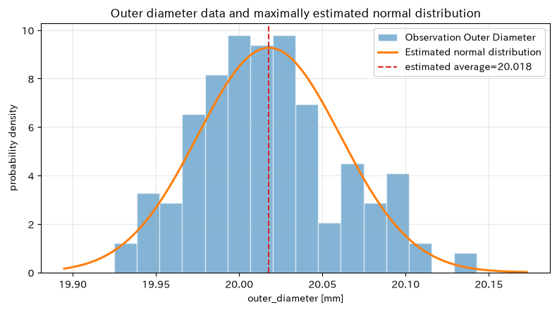
plt.hist(diameter, bins=16, density=True, alpha=0.55, edgecolor="white", label="Observation Outer Diameter")
plt.plot(x_grid, stats.norm.pdf(x_grid, mu_hat, sigma_hat), lw=2.2, label="Estimated normal distribution")
plt.axvline(mu_hat, color="tab:red", ls="--", label=f"estimated average={mu_hat:.3f}")
plt.title("Outer diameter data and maximally estimated normal distribution")
plt.xlabel("outer_diameter [mm]")
plt.ylabel("probability density")
plt.grid(True, alpha=0.3)
plt.legend()
plt.tight_layout()
plt.show()

	Estimated Subject	Most likelihood estimate	Unit
0	average mu	20.0179	mm
1	standard_deviation sigma	0.0430	mm

Reading the results

The estimated average is not the standard value itself, but rather the process center most supported by this sample. You can visually see that the histogram and estimation curve do not differ significantly, but this does not guarantee normality. Process adjustment is not determined solely by averages; changes in specification limits, measurement errors, time-series drift, and standard deviations are also checked.

No.042: Maximum likelihood estimation (binomial distribution) — estimating the misfit rate across lots

Meaning in Practice

From the number of inspections $n_j$ and the number of nonconformities $k_j$ for lot $j$, the common probability of nonconformance $p$ is estimated. In simple average lot rates, the number of lots inspected is overweighted, so the total number of items inspected is aggregated as the standard.

Approach to Analysis and Modeling

$K=\sum_j k_j$, if $N=\sum_j n_j$ is the binomial likelihood is $L(p)\propto p^K(1-p)^{N-K}$, and the maximum likelihood estimate is

$\hat p=\frac{K}{N}$

That’s right. This is based on the assumption that the probability of nonconformity among individual individuals is common and independent. If rates differ among process, product, or inspector, stratification or regression models are necessary.

Check with Python

total_defects = defect_counts.sum()
total_inspected = lot_sizes.sum()
p_hat = total_defects / total_inspected
lot_rates = defect_counts / lot_sizes

binomial_result = pd.DataFrame({
    "indicator": ["Total number of inspections", "Total number of nonconformities", "binomialMLE", "Simple average of lot rates"],
    "value": [total_inspected, total_defects, p_hat, lot_rates.mean()],
})
display(binomial_result.round(5))

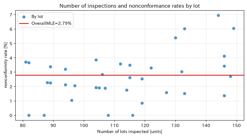
plt.scatter(lot_sizes, lot_rates * 100, alpha=0.75, label="By lot")
plt.axhline(p_hat * 100, color="tab:red", lw=2, label=f"OverallMLE={p_hat:.2%}")
plt.title("Number of inspections and nonconformance rates by lot")
plt.xlabel("Number of lots inspected [units]")
plt.ylabel("nonconformity rate [%]")
plt.grid(True, alpha=0.3)
plt.legend()
plt.tight_layout()
plt.show()

	indicator	value
0	Total number of inspections	4079.00000
1	Total number of nonconformities	114.00000
2	binomialMLE	0.02795
3	Simple average of lot rates	0.02672

Reading the results

Binomial MLE is the “total number of nonconformities ÷ total number of inspections,” and is a weighted average based on the number of inspections. The scatter plot also shows that the fewer lots inspected, the more likely the rate to fluctuate discretely. It is safer not to rank lots based solely on this overall rate; instead, it is safer to check the process conditions and confidence intervals for each lot.

No.043: Maximum Likelihood Estimation (Poisson Distribution) — Estimating the daily incidence rate of sudden stops

Meaning in Practice

Relatively rare events that occur within a certain period include the number of stoppages, failures, and defects. Estimating the average daily incidence rate of $\lambda$ serves as a basis for considering the required number of maintenance personnel and spare parts.

Approach to Analysis and Modeling

$Y_i\sim\mathrm{Poisson}(\lambda)$ Then,

$P(Y_i=y_i)=\frac{e^{-\lambda}\lambda^{y_i}}{y_i!},\qquad \hat\lambda=\bar y$

That’s right. The Poisson distribution strongly assumes that the mean and variance are equal. If there is overdistribution, zero overload, day of the week effect, or consecutive failures, consider a different model.

Check with Python

lambda_hat = stoppages.mean()
poisson_check = pd.DataFrame({
    "indicator": ["Average (lambda MLE）", "sample dispersion", "disperse / average", "Percentage of Zero Downtime Days"],
    "value": [lambda_hat, stoppages.var(ddof=1), stoppages.var(ddof=1) / lambda_hat, np.mean(stoppages == 0)],
})
display(poisson_check.round(3))

k = np.arange(0, stoppages.max() + 1)
observed = np.bincount(stoppages, minlength=len(k))[:len(k)] / len(stoppages)
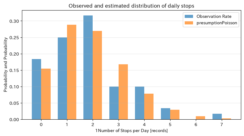
plt.bar(k - 0.18, observed, width=0.36, alpha=0.7, label="Observation Rate")
plt.bar(k + 0.18, stats.poisson.pmf(k, lambda_hat), width=0.36, alpha=0.7, label="presumptionPoisson")
plt.title("Observed and estimated distribution of daily stops")
plt.xlabel("1Number of Stops per Day [records]")
plt.ylabel("Probability and Probability")
plt.grid(True, axis="y", alpha=0.3)
plt.legend()
plt.tight_layout()
plt.show()

	indicator	value
0	Average (lambda MLE）	1.867
1	sample dispersion	2.219
2	disperse / average	1.189
3	Percentage of Zero Downtime Days	0.183

Reading the results

The average number of stops is the most likely estimate. If ÷ sample variance means deviates significantly from 1, we doubt the assumption of a single constant incidence. The incidence rate obtained here is a candidate input for the staffing plan, but since the “recovery time per case” is not included, a downtime model is also necessary for the workload plan.

No.044: Optimization with scipy.optimize — Implementing constrained numerical estimation

Meaning in Practice

In standard distributions, estimates can be written by formulas, but if there are cut-offs, multiple factors, or complex constraints, closed forms may not be obtained. By using numerical optimization, you can solve with negative logarithmic likelihood as the objective function and within the same framework.

Approach to Analysis and Modeling

Maximization replaces the minimization of $-\ell(\theta)$. Optimize the $\eta=\log\sigma$ to ensure the $\sigma>0$ is met, and finally return to the $\sigma=e^\eta$. Checking initial values, scaling, convergence flags, and boundary solutions is practically important.

Check with Python

def normal_nll(params, x):
    mu, log_sigma = params
    sigma = np.exp(log_sigma)
    return -np.sum(stats.norm.logpdf(x, loc=mu, scale=sigma))

opt_result = minimize(
    normal_nll,
    x0=np.array([20.0, np.log(0.05)]),
    args=(diameter,),
    method="Nelder-Mead",
    options={"xatol": 1e-11, "fatol": 1e-11, "maxiter": 2000},
)
mu_opt, sigma_opt = opt_result.x[0], np.exp(opt_result.x[1])
optimization_check = pd.DataFrame({
    "item": ["convergence", "Number of repetitions", "Optimization mu", "analytical solution mu", "Optimization sigma", "analytical solution sigma"],
    "value": [opt_result.success, opt_result.nit, mu_opt, mu_hat, sigma_opt, sigma_hat],
})
optimization_check

	item	value
0	convergence	True
1	Number of repetitions	77
2	Optimization mu	20.017902
3	analytical solution mu	20.017902
4	Optimization sigma	0.043047
5	analytical solution sigma	0.043047

Reading the results

If the numerical solution roughly matches the analysis solution in No.041, you can check the implementation of the objective function and variable transformation. Not only success, but also check whether the initial value is changed to reach the same solution, whether the gradient is sufficiently small, and whether it is within a range that is possible for the job. Optimizers do not guarantee the validity of the model.

No.045: Visualizing the likelihood function — Seeing the uncertainty around the estimate

Meaning in Practice

The maximum likelihood estimate is single, but candidates with close likelihood also match the data. By looking at the likelihood range, you can intuitively determine how many decimal places the process mean can be discussed and whether additional measurements are needed.

Approach to Analysis and Modeling

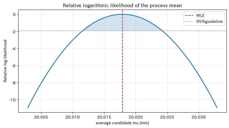
$\sigma$ fixed as an estimate, and the relative logarithmic likelihood for each candidate $\mu$

$\ell(\mu)-\ell(\hat\mu)$

Draw. For a one-parameter likelihood ratio approximation, the 95% guideline is $-\chi^2_{1,0.95}/2\approx-1.92$. This is a finite sample and not necessarily a precise interval.

Check with Python

mu_candidates = np.linspace(mu_hat - 0.015, mu_hat + 0.015, 301)
loglik = np.array([
    np.sum(stats.norm.logpdf(diameter, loc=mu, scale=sigma_hat))
    for mu in mu_candidates
])
relative_loglik = loglik - loglik.max()
cutoff = -stats.chi2.ppf(0.95, df=1) / 2
supported = mu_candidates[relative_loglik >= cutoff]

print(f"By likelihood ratio95%Support Range (Approximate): {supported.min():.5f} ～ {supported.max():.5f} mm")
plt.plot(mu_candidates, relative_loglik, lw=2)
plt.axvline(mu_hat, color="tab:red", ls="--", label="MLE")
plt.axhline(cutoff, color="tab:gray", ls=":", label="95%guideline")
plt.fill_between(mu_candidates, relative_loglik, cutoff,
                 where=relative_loglik >= cutoff, alpha=0.2)
plt.title("Relative logarithmic likelihood of the process mean")
plt.xlabel("average candidate mu [mm]")
plt.ylabel("Relative log-likelihood")
plt.grid(True, alpha=0.3)
plt.legend()
plt.tight_layout()
plt.show()

95% support range by likelihood ratio (approximate): 20.01170 ~ 20.02410 mm

Reading the results

If the vertex of the curve is the maximum likelihood estimate and the area near the vertex is flat, it is harder to narrow down candidates; if sharp, the accuracy is higher. If the support range is wider than what is manageably acceptable, it leads to decisions to increase the number of measurements and avoid excessive fine-tuning. Note that the purpose differs from the standard conformity assessment section.

No.046: Gradient Calculation — Checking the Direction in Which Likelihood Improves

Meaning in Practice

The gradient is “how much the objective function changes when the parameters are slightly changed.” It helps diagnose why optimization has stopped, verify the implementation of proprietary models, and understand the direction of updates to online estimates.

Approach to Analysis and Modeling

The gradient of the negative logarithmic likelihood $J(\mu)$ of a normal distribution fixed $\sigma$ is

$$\frac{dJ}{d\mu}=\frac{n\mu-\sum_i x_i}{\sigma^2}$$

That’s right. Compare with the central difference $(J(\mu+h)-J(\mu-h))/(2h)$ and check the formula and code. At the most critical point, the gradient is almost zero.

Check with Python

def nll_mu(mu):
    return -np.sum(stats.norm.logpdf(diameter, loc=mu, scale=sigma_hat))

def analytic_gradient(mu):
    return (len(diameter) * mu - diameter.sum()) / sigma_hat**2

h = 1e-6
check_points = np.array([mu_hat - 0.006, mu_hat, mu_hat + 0.006])
gradient_table = pd.DataFrame({
    "muCandidate": check_points,
    "analytical gradient": [analytic_gradient(mu) for mu in check_points],
    "Numerical gradient": [(nll_mu(mu + h) - nll_mu(mu - h)) / (2 * h) for mu in check_points],
})
gradient_table["absolute value of difference"] = abs(gradient_table["analytical gradient"] - gradient_table["Numerical gradient"])
gradient_table.round(6)

	muCandidate	analytical gradient	Numerical gradient	absolute value of difference
0	20.011902	-582.825624	-582.825624	0.000001
1	20.017902	0.000000	-0.000000	0.000000
2	20.023902	582.825624	582.825625	0.000001

Reading the results

If the analytical gradient and numerical gradient are close, it can be judged that there are no major errors in the implementation of the differential formula. To the left of the MLE it is negative, and to the right it is positive, so the direction of lowering the negative logarithmic likelihood is toward the center. If the difference width is too small, it results in rounding error; if too large, the approximate error increases, so check with multiple widths.

No.047: Newton’s Method — Repeatedly estimating the Stop Rate Using Curvature

Meaning in Practice

Newton’s method uses not only gradients but also curvature, approaching the solution in an iterative manner. By keeping update histories in the example of the daily downtime rate, the implementation allows not only the “answer” but also the convergence process to be audited.

Approach to Analysis and Modeling

The first- and second-order differentiations of Poisson log-likelihood are

$$\ell'(\lambda)=\frac{\sum_i y_i}{\lambda}-n,\qquad \ell''(\lambda)=-\frac{\sum_i y_i}{\lambda^2}$$

That’s right. Use the update $\lambda_{t+1}=\lambda_t-\ell'(\lambda_t)/\ell''(\lambda_t)$. For complex problems that may break positive constraints, step control and logarithmic transformation are necessary.

Check with Python

lam = 0.6
history = []
sum_y, n_days = stoppages.sum(), len(stoppages)
for iteration in range(1, 9):
    score = sum_y / lam - n_days
    curvature = -sum_y / lam**2
    new_lam = lam - score / curvature
    history.append((iteration, lam, score, new_lam))
    if abs(new_lam - lam) < 1e-10:
        lam = new_lam
        break
    lam = new_lam

newton_history = pd.DataFrame(history, columns=["Repeatedly", "Before updatelambda", "Score", "After the updatelambda"])
display(newton_history.round(6))
print(f"Newtonlaw={lam:.6f}, Analytical solution (sample mean)={lambda_hat:.6f}")

	Repeatedly	Before updatelambda	Score	After the updatelambda
0	1	0.600000	126.666667	1.007143
1	2	1.007143	51.205674	1.470891
2	3	1.470891	16.144322	1.782753
3	4	1.782753	2.824173	1.862894
4	5	1.862894	0.121495	1.866659
5	6	1.866659	0.000245	1.866667
6	7	1.866667	0.000000	1.866667

Newton's method = 1.866667, analytical solution (sample mean) = 1.866667

Reading the results

The updated value converges to the sample mean and matches No.043. Comparing simple examples with analytical solutions is an important test before moving on to more complex likelihood values. In the practical system, logs record the maximum number of iterations, tolerance of error, non-finite values, improvements to objective functions, and handling when not converging.

No.048: Fisher Information Amount — Linking Measurement Numbers with Estimation Accuracy

Meaning in Practice

Increasing measurement improves accuracy, but also increases costs. The Fisher information quantity quantifies the information the observation holds about unknown parameters, supporting discussions on test design and the required sample size.

Approach to Analysis and Modeling

For a normal mean where the standard deviation $\sigma$ is known,

$I_n(\mu)=\frac{n}{\sigma^2},\qquad \mathrm{SE}(\hat\mu)\approx\frac{1}{\sqrt{I_n}}=\frac{\sigma}{\sqrt n}$

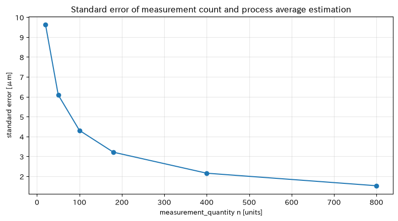
That’s right. To halve the standard error, the number of measurements needs to be four times higher. If the conditions of independent identical distribution, model fit, and known parameters are excluded, the formula for information quantity also changes.

Check with Python

sample_sizes = np.array([20, 50, 100, 180, 400, 800])
fisher_info = sample_sizes / sigma_hat**2
standard_error = 1 / np.sqrt(fisher_info)
fisher_table = pd.DataFrame({
    "measurement_quantity n": sample_sizes,
    "Fisheramount of information": fisher_info,
    "Standard error of average estimation [mm]": standard_error,
    "similar95%half-width [mm]": 1.96 * standard_error,
})
display(fisher_table.round(6))

plt.plot(sample_sizes, standard_error * 1000, marker="o")
plt.title("Standard error of measurement count and process average estimation")
plt.xlabel("measurement_quantity n [units]")
plt.ylabel("standard error [μm]")
plt.grid(True, alpha=0.3)
plt.tight_layout()
plt.show()

	measurement_quantity n	Fisheramount of information	Standard error of average estimation [mm]	similar95%half-width [mm]
0	20	10793.067110	0.009626	0.018866
1	50	26982.667774	0.006088	0.011932
2	100	53965.335549	0.004305	0.008437
3	180	97137.603988	0.003209	0.006289
4	400	215861.342195	0.002152	0.004219
5	800	431722.684389	0.001522	0.002983

Reading the results

As the number of measurements increases, the standard error decreases by only $1/\sqrt n$, resulting in a marginal effect. Practically, it is necessary to calculate the sample size backward from the required accuracy and compare it with measurement costs and decision losses. For continuous measurements with autocorrelation, the effective sample size is smaller, so this table cannot be used as is.

No.049: Bootstrap — Evaluating Uncertainty in Process Averages by Resampling

Meaning in Practice

For complex KPIs or statistics that are difficult to set theoretical distributions, deriving formulas for standard error is challenging. The bootstrap repeatedly extracts and reconstructs from observation samples, evaluating variation in estimates and intervals.

Approach to Analysis and Modeling

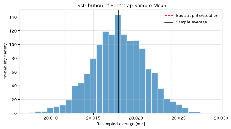
Samples of the same size are reconstructed and extracted from the original sample, and the average is calculated for each sample. Here, we calculate the 95% interval using the percentile method of 3,000 operations. It is assumed that the observation specimen represents the population and that the observation units are interchangeable. Time series and lot structures require block-by-block resampling.

Check with Python

n_boot = 3000
bootstrap_samples = rng.choice(diameter, size=(n_boot, len(diameter)), replace=True)
bootstrap_means = bootstrap_samples.mean(axis=1)
boot_ci = np.quantile(bootstrap_means, [0.025, 0.975])
theory_ci = mu_hat + np.array([-1, 1]) * stats.t.ppf(0.975, len(diameter)-1) * diameter.std(ddof=1) / np.sqrt(len(diameter))

ci_table = pd.DataFrame({
    "Methods": ["Bootstrap percentile", "tsimilar"],
    "lower_limit [mm]": [boot_ci[0], theory_ci[0]],
    "upper [mm]": [boot_ci[1], theory_ci[1]],
})
display(ci_table.round(5))

plt.hist(bootstrap_means, bins=30, density=True, alpha=0.7, edgecolor="white")
plt.axvline(boot_ci[0], color="tab:red", ls="--", label="Bootstrap 95%section")
plt.axvline(boot_ci[1], color="tab:red", ls="--")
plt.axvline(mu_hat, color="black", lw=1.8, label="Sample Average")
plt.title("Distribution of Bootstrap Sample Mean")
plt.xlabel("Resampled average [mm]")
plt.ylabel("probability density")
plt.grid(True, alpha=0.3)
plt.legend()
plt.tight_layout()
plt.show()

	Methods	lower_limit [mm]	upper [mm]
0	Bootstrap percentile	20.01178	20.02422
1	tsimilar	20.01155	20.02425

Reading the results

If the bootstrap interval and the t-approximation interval are close, the difference in method choice can be considered small in this data. However, the interval is an uncertainty in the process average and does not fall within the scope of individual product dimensions. Abnormal modes and future process changes not included in the sample cannot be reproduced, so they cannot replace data collection design.

No.050: EM Algorithm — Estimating Mixing Processes Without Equipment ID

Meaning in Practice

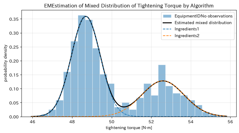
Missing equipment IDs or merging processes can cause measurements from different states to be mixed. Simply using the overall average can lead to mistaking the difference between two normal facilities as “large variation.” The EM algorithm repeatedly estimates the mixing ratio, mean, and standard deviation from data where the affiliation is not visible.

Approach to Analysis and Modeling

Two-component normal mixing model

$p(x)=\sum_{k=1}^{2}\pi_k\,N(x\mid\mu_k,\sigma_k^2)$

Let’s assume the following assumptions. The E-step calculates the probability of belonging (responsibility), and the M-step uses that probability as a weight to update the $\pi_k,\mu_k,\sigma_k$. The mixed number is not automatically determined, and since there are local solutions and label replacements, multiple initial values and operational knowledge are required.

Check with Python

def em_two_normals(x, max_iter=200, tol=1e-8):
    means = np.quantile(x, [0.3, 0.7]).astype(float)
    sigmas = np.array([x.std(), x.std()])
    weights = np.array([0.5, 0.5])
    loglik_history = []

    for _ in range(max_iter):
        weighted_pdf = np.column_stack([
            weights[k] * stats.norm.pdf(x, means[k], sigmas[k]) for k in range(2)
        ])
        denominator = weighted_pdf.sum(axis=1, keepdims=True)
        responsibilities = weighted_pdf / denominator
        nk = responsibilities.sum(axis=0)
        weights = nk / len(x)
        means = (responsibilities * x[:, None]).sum(axis=0) / nk
        sigmas = np.sqrt(
            (responsibilities * (x[:, None] - means)**2).sum(axis=0) / nk
        )
        loglik = np.log(denominator[:, 0]).sum()
        loglik_history.append(loglik)
        if len(loglik_history) > 1 and abs(loglik_history[-1] - loglik_history[-2]) < tol:
            break

    order = np.argsort(means)
    return weights[order], means[order], sigmas[order], np.array(loglik_history), responsibilities[:, order]

em_weights, em_means, em_sigmas, em_loglik, responsibilities = em_two_normals(torque)
em_result = pd.DataFrame({
    "presumed component": ["Low torque side", "High Torque Side"],
    "Mixing ratio": em_weights,
    "average [N·m]": em_means,
    "standard_deviation [N·m]": em_sigmas,
})
display(em_result.round(3))
print(f"Number of repetitions: {len(em_loglik)}, final log-likelihood: {em_loglik[-1]:.2f}")

x_grid = np.linspace(torque.min() - 0.5, torque.max() + 0.5, 400)
mixture_pdf = sum(
    em_weights[k] * stats.norm.pdf(x_grid, em_means[k], em_sigmas[k]) for k in range(2)
)
plt.hist(torque, bins=24, density=True, alpha=0.5, edgecolor="white", label="equipmentIDNo observations")
plt.plot(x_grid, mixture_pdf, color="black", lw=2.2, label="Estimated mixed distribution")
for k, color in enumerate(["tab:blue", "tab:orange"]):
    plt.plot(x_grid, em_weights[k] * stats.norm.pdf(x_grid, em_means[k], em_sigmas[k]),
             color=color, ls="--", label=f"Ingredients{k+1}")
plt.title("EMEstimation of Mixed Distribution of Tightening Torque by Algorithm")
plt.xlabel("tightening torque [N·m]")
plt.ylabel("probability density")
plt.grid(True, alpha=0.3)
plt.legend()
plt.tight_layout()
plt.show()

	presumed component	Mixing ratio	average [N·m]	standard_deviation [N·m]
0	Low torque side	0.657	48.692	0.731
1	High Torque Side	0.343	52.592	1.071

Number of iterations: 34, Final log-likeness: -589.01

Reading the results

Rather than treating the entire process as a single distribution, process states can be explained as two components: the low-torque side and the high-torque side. However, the conclusion that components correspond to actual equipment requires restoration and verification of maintenance records and equipment IDs. EM does not identify causality and depends on initial values and the number of components. First, prioritize improving traceability, and use EM as an auxiliary analysis for the loss period.

Practical Implications Seen Through Target Exercise

1. Report estimates and uncertainties together: Focusing solely on average or rate alone does not determine the priority for adjustment, maintenance, or additional inspections.
2. Mapping the generation mechanism to the data type: The likelihood varies depending on the continuous amount, pass/fail, and number of cases, so the required assumptions also change.
3. Cross-checking analytical and numerical solutions: Confirming matches in simple cases can enhance the reliability of complex implementations.
4. Measure the number based on the required accuracy: Design based on acceptable estimation errors and decision costs, rather than conventional extracts.
5. Mixed distributions can sometimes indicate data management issues: Before supplementing with advanced estimations, establish identifiers for equipment, materials, and working conditions.

The output of the statistical model is not an automatic action command. Only by linking process knowledge, standards, losses, and change management can it be used for decision-making.

What is necessary for practical implementation

• Defining Purpose and Decision-Making: Clearly state what is estimated and who judges what at which threshold
• Checking the measurement system: Evaluate calibration, resolution, repeatability, and reproducibility, and grasp measurement errors
• Data Contracts and Tier Keys: Coordinate equipment, molds, material lots, shifts, inspectors, and time without missing any gaps.
• Model Diagnosis: Check independence, homeostasis, distribution fit, overdispersion, outliers, and mixed states
• Verification and Monitoring: Conduct period-specific reproducibility checks and continuous monitoring of estimates, intervals, convergence logs, and data quality.
• Operations Design: Establish escalation, relearning, approval, rollback, and audit trails in case of abnormalities

It is safer to start with small-scale target processes running in parallel with current decisions. We evaluate not only estimation accuracy but also operational KPIs including missed items, over-adjustments, and inspection man-hours.

Conclusion

From No.041 to No.050, starting from the maximum likelihood estimation of normal, binomial, and Poisson models, we implemented numerical optimization using SciPy, likelihood shapes, gradients, Newton’s method, Fisher information content, bootstraps, and EM algorithms.

The core idea is not just to find the parameters that best match the observed values, but to Simultaneously checking assumptions, estimation accuracy, convergence, and data generation processes. When introducing to manufacturing sites, improving model accuracy is just as important as establishing measurement systems, layer keys, decision rules, and monitoring systems.

Consultations for Corporations

At Surikoubo, we support everything from quality data analysis, statistical model construction, inspection design, equipment maintenance analysis, Python training, and PoC to operational implementation in manufacturing. You can consult from stages such as “wanting to take a step beyond aggregating average values,” “converting estimated results into on-site criteria,” or “having issues with equipment labels or data quality.”

📩 Contact Us: surikobo.co.jp/contact
Please feel free to consult us first.