Updating Uncertainty and Choosing Improvements: 10 Bayesian Statistics in Manufacturing Exercise

On the manufacturing floor, nonconformity rates and downtime are estimated from limited observations, and additional inspections, process changes, and improvement plans are decided. In this article, we will use a fictional precision parts factory as the subject and implement How to Integrate Prior Distribution and Observational Data to Update Uncertainty in a continuous sequence, including Beta Bernoulli, Gamma Poissons, MCMC, PyMC, hierarchical Bayesian, predictive distribution, and Bayesian A/B testing.

The value of Bayesian statistics is not simply about “estimating the average.” It means being able to answer questions directly related to decision-making, such as “The probability that the nonconformity rate exceeds management standards,” “How many incidents will occur next week?” and “The probability that improvement proposals will be better than the current ones.” On the other hand, since results depend on prior distributions and model assumptions, sensitivity analysis and operational design are essential.

[!NOTE] This material is a notebook previously used by Surikoubo (or personally by the representative, Kazuyama), and has been reconstructed, edited, and published with the company’s permission. All data listed is fictional and has no relation whatsoever to real companies, factories, or figures.

Introduction: Practical Challenges in Manufacturing Covered in This Article

Consider a scenario in a fictional precision valve factory where the quality assurance department and equipment maintenance team decide on measures for the following month. The Quality Assurance Department determines whether seal nonconformities have decreased under the new cleaning conditions, and the maintenance team estimates the number of personnel needed to prepare for sudden shutdowns. Additionally, a system is needed to compare the performance of multiple factories and avoid excessively evaluating or criticizing those with limited data.

What is needed here is not a single estimate, but a probability distribution of unknown quantities. Each time observations increase, the distribution is updated, and from that distribution, the probability of exceedance, the number of forecasts, and the probability of the measure being superior are calculated.

Common situations on site

• Report the nonconformance rate only as one point: ‘Number of Nonconformances ÷ Number of Inspections,’ and compare while ignoring differences in parameters.
• Although there is past experience and knowledge of similar processes, it is only used as a hunch by the person in charge
• Even when data is added, monthly materials are simply recreated, and update rules are not standardized.
• Without confirming simulation convergence or effective sample size, only the average value of MCMC is used.
• They do not distinguish between ‘the improved version seems better’ and ‘the improvements have met investment criteria.‘

Why is this issue so difficult to judge?

Even if there are zero nonconformities, if there are 10 tests, it cannot be said that the “true nonconformance rate is 0%.” Conversely, if you place too much emphasis on past insights, even if data shows process changes, updates will be delayed. Bayes’ theorem states that for an unknown parameter $\theta$,

$$p(\theta\mid y)=\frac{p(y\mid\theta)p(\theta)}{p(y)} \propto p(y\mid\theta)p(\theta)$$

This is how it is expressed. $p(\theta)$ is the prior distribution, $p(y\mid\theta)$ is the likelihood, and $p(\theta\mid y)$ is the posterior distribution. It is necessary to clearly define not only the formulas but also who and which information the prior distribution represents, whether the data generation process is valid, and which probabilities should be used as decision-making criteria.

Overview of Exercise covered this time

No.	Theme	Questions in the Manufacturing Industry
071	Beta Bernoulli	What range should the seal nonconformance rate be considered?
072	Gamma Poisson	What is the daily equipment downtime rate?
073	Bayes Update	How decisions change with each additional lot
074	MCMC	Can posterior distributions be approximated without using analytical solutions?
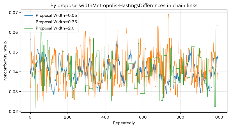
075	Metropolis-Hastings	How proposal width and acceptance rate affect estimated quality?
076	Gibbs Sampling	Can you alternate between estimating averages and variation?
077	Introduction to PyMC	Can declarative models estimate the rate of nonconformance?
078	hierarchical Bayes	How to stabilize a small amount of data per factory
079	Bayesian Prediction Distribution	What is the probability that the next test will exceed the standard?
080	Bayesian A/B Test	Is there sufficient grounds for implementing the new conditions?

Preparing the Python environment

NumPy is used for random number and numerical calculations, pandas for tables, SciPy for probability distributions, matplotlib for visualization, and No.077 uses PyMC. Japanese use japanize_matplotlib for display. External data and seaborn are not used. Fix random seed numbers so that the same results can be reproduced in the same environment.

import platform
import warnings

import numpy as np
import pandas as pd
import scipy
from scipy import stats
from scipy.special import betaln, expit
import matplotlib
import matplotlib.pyplot as plt
import japanize_matplotlib
import pytensor
pytensor.config.cxx = ""  # Uses a Python implementation that can run even in environments without a C++ toolchain.
import pymc as pm
from IPython.display import display

warnings.filterwarnings("ignore", category=FutureWarning)
pd.set_option("display.precision", 4)
plt.rcParams["figure.figsize"] = (8, 4.5)
plt.rcParams["axes.unicode_minus"] = False

SEED = 20260711
rng = np.random.default_rng(SEED)

pd.DataFrame({
    "item": ["Python", "NumPy", "pandas", "SciPy", "matplotlib", "PyMC", "random numberseed"],
    "value": [platform.python_version(), np.__version__, pd.__version__, scipy.__version__,
           matplotlib.__version__, pm.__version__, SEED],
})

	item	value
0	Python	3.13.1
1	NumPy	2.5.1
2	pandas	3.0.3
3	SciPy	1.18.0
4	matplotlib	3.11.0
5	PyMC	5.26.1
6	random numberseed	20260711

Creation of Fictional Data

Assuming multiple decisions within the same factory, (1) seal inspection for 12 lots, (2) number of equipment stoppages over 35 days, (3) filling time, (4) inspection records of 6 factories, and (5) comparative data between current and new cleaning conditions. In practice, it is confirmed that processes, equipment, materials, and measurement methods have not changed during the period, and if there are changes, stratification or time-varying models are considered.

# Seal inspection: The number of inspections varies by lot
lot_n = rng.integers(45, 76, size=12)
lot_defects = rng.binomial(lot_n, 0.038)
inspection_df = pd.DataFrame({
    "lot": [f"L{i:02d}" for i in range(1, 13)],
    "number_of_inspections": lot_n,
    "non_conforming_number": lot_defects,
})
inspection_df["nonconformity rate"] = inspection_df["non_conforming_number"] / inspection_df["number_of_inspections"]

# Equipment shutdown, filling time, factory-specific inspections, A/B comparison
daily_stops = rng.poisson(1.35, size=35)
fill_time = rng.normal(42.4, 1.8, size=45)
plant_names = ["Northeast", "Kanto", "Central region", "Kansai", "China", "Kyushu"]
plant_n = np.array([80, 520, 140, 950, 65, 300])
plant_true_p = np.array([0.042, 0.031, 0.050, 0.027, 0.060, 0.036])
plant_k = rng.binomial(plant_n, plant_true_p)
ab_n = {"Current Conditions": 650, "New Cleaning Conditions": 620}
ab_k = {
    "Current Conditions": rng.binomial(ab_n["Current Conditions"], 0.046),
    "New Cleaning Conditions": rng.binomial(ab_n["New Cleaning Conditions"], 0.028),
}

display(inspection_df)
display(pd.DataFrame({
    "Data": ["equipment shutdown", "filling time", "Factory-specific inspections", "A/BComparison"],
    "Observation Scale": [f"{len(daily_stops)}days", f"{len(fill_time)}units", f"{len(plant_names)}Factory",
             f"{sum(ab_n.values())}units"],
}))

	lot	number_of_inspections	non_conforming_number	nonconformity rate
0	L01	71	1	0.0141
1	L02	51	4	0.0784
2	L03	50	2	0.0400
3	L04	73	2	0.0274
4	L05	47	3	0.0638
5	L06	61	2	0.0328
6	L07	64	3	0.0469
7	L08	65	3	0.0462
8	L09	72	3	0.0417
9	L10	71	1	0.0141
10	L11	55	2	0.0364
11	L12	51	3	0.0588

	Data	Observation Scale
0	equipment shutdown	35days
1	filling time	45units
2	Factory-specific inspections	6Factory
3	A/BComparison	1270units

No.071: Beta Bernoulli — Estimating the Rate of Nonconformity by Distribution

Meaning in Practice

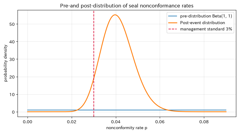
If individual products are represented as conformity 0 or non-conformance 1, the unknown nonconformance rate $p$ can be treated as the Bernoulli probability. In addition to point estimation, you can determine the priority for additional tests and cause investigations by determining the $p$‘s credit range and the ‘probability of exceeding the 3% management standard.‘

Approach to Analysis and Modeling

If we $p\sim\mathrm{Beta}(\alpha_0,\beta_0)$ the prior distribution, $k$ the number of observed nonconformities, and $n$ the number of tests, then by conjugation,

$$p\mid k,n\sim\mathrm{Beta}(\alpha_0+k,\ \beta_0+n-k)$$

That’s right. Here, we place the weak pre-distribution $\mathrm{Beta}(1,1)$. When using past results in practice, the period, equipment, and product families used as the basis should be listed together with the effective sample size $\alpha_0+\beta_0$ of the prior distribution.

Check with Python

n_total = int(inspection_df["number_of_inspections"].sum())
k_total = int(inspection_df["non_conforming_number"].sum())
a0, b0 = 1.0, 1.0
a_post, b_post = a0 + k_total, b0 + n_total - k_total
ci71 = stats.beta.ppf([0.025, 0.975], a_post, b_post)
threshold = 0.03

beta_summary = pd.DataFrame({
    "indicator": ["number_of_inspections", "non_conforming_number", "Observation rate", "Post-event average", "95%Lower limit of the credit range", "95%Credit Bracket Limit", "P(p > 3%)"],
    "value": [n_total, k_total, k_total/n_total, a_post/(a_post+b_post), *ci71,
           stats.beta.sf(threshold, a_post, b_post)],
})
display(beta_summary)

x = np.linspace(0, 0.09, 500)
plt.plot(x, stats.beta.pdf(x, a0, b0), label="pre-distribution Beta(1, 1)")
plt.plot(x, stats.beta.pdf(x, a_post, b_post), label="Post-event distribution", linewidth=2)
plt.axvline(threshold, color="crimson", linestyle="--", label="management standard 3%")
plt.title("Pre-and post-distribution of seal nonconformance rates")
plt.xlabel("nonconformity rate p")
plt.ylabel("probability density")
plt.grid(alpha=0.3)
plt.legend()
plt.tight_layout()
plt.show()

	indicator	value
0	number_of_inspections	731.0000
1	non_conforming_number	29.0000
2	Observation rate	0.0397
3	Post-event average	0.0409
4	95%Lower limit of the credit range	0.0278
5	95%Credit Bracket Limit	0.0564
6	P(p > 3%)	0.9437

Reading the results

The posterior average is the smoothed value of the current nonconformity rate, and the 95% credit interval is the range where unknown $p$ have a 95% probability under the model and prior distribution. If the post-event probability exceeds 3% of the management standard, it provides grounds not only for simple pass/fail judgments but also for prioritizing additional inspections and stratification of process factors. However, this probability depends on the assumption that the same $p$ will continue between lots.

No.072: Gamma Poison — Updating the Rate of Equipment Outages

Meaning in Practice

By modeling the daily number of sudden shutdowns, you can probabilistically estimate the required amounts of maintenance shifts, spare parts, and recovery support. To handle not only the presence or absence of stops but also the number of cases, the incidence rate $\lambda$ is estimated over a certain period.

Approach to Analysis and Modeling

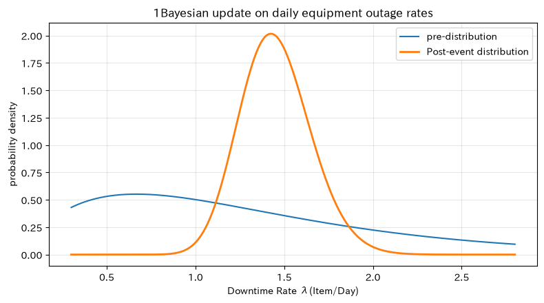
$y_t\sim\mathrm{Poisson}(\lambda)$, if the pre-distribution of rate parameter representation is $\lambda\sim\mathrm{Gamma}(a_0,b_0)$, the post-post distribution observed for the total number of cases over $T$ days $\sum y_t$ is

$$\lambda\mid y\sim\mathrm{Gamma}\left(a_0+\sum_{t=1}^{T}y_t,\ b_0+T\right)$$

That’s right. Note that SciPy’s scale is specified as the reciprocal of the rate $1/b$.

Check with Python

ga, gb = 2.0, 1.5  # Average advance rate: 1.33 cases/day
ga_post = ga + daily_stops.sum()
gb_post = gb + len(daily_stops)
lambda_mean = ga_post / gb_post
lambda_ci = stats.gamma.ppf([0.025, 0.975], ga_post, scale=1/gb_post)

display(pd.DataFrame({
    "indicator": ["Observation Days", "Total number of stoppages", "specimen mean", "Post-event average", "95%Lower limit of the credit range", "95%Credit Bracket Limit"],
    "value": [len(daily_stops), daily_stops.sum(), daily_stops.mean(), lambda_mean, *lambda_ci],
}))

lam_x = np.linspace(0.3, 2.8, 500)
plt.plot(lam_x, stats.gamma.pdf(lam_x, ga, scale=1/gb), label="pre-distribution")
plt.plot(lam_x, stats.gamma.pdf(lam_x, ga_post, scale=1/gb_post), label="Post-event distribution", linewidth=2)
plt.title("1Bayesian update on daily equipment outage rates")
plt.xlabel("Downtime Rate λ(Item/Day)")
plt.ylabel("probability density")
plt.grid(alpha=0.3)
plt.legend()
plt.tight_layout()
plt.show()

	indicator	value
0	Observation Days	35.0000
1	Total number of stoppages	51.0000
2	specimen mean	1.4571
3	Post-event average	1.4521
4	95%Lower limit of the credit range	1.0877
5	95%Credit Bracket Limit	1.8682

Reading the results

The close sampling mean and post-poster mean are because 35 days of observations are more effective than weak prior data. Credit zones indicate the dangers of fixing a conservation plan at a single point. However, the Poisson distribution assumes a constant daily incidence rate and equal variance with the mean. If overvariance occurs in the chain of days of the week, variety, uptime, or failures, it is extended to negative binomial models or models that include covariates.

No.073: Bayes Update — Update judgments every lot arrival

Meaning in Practice

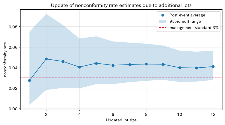
Not only can all data be consolidated at the end of the month, but by updating the distribution of nonconformance rates after each lot inspection, you can speed up decisions on additional inspections or process stoppages. By keeping update history, you can explain when and on what data your decisions changed.

Approach to Analysis and Modeling

The beta distribution parameters can be interpreted as the “number of pseudo-cases on the non-conforming side” and “number of pseudo-cases on the conforming side.” Sequential updates that change the post-distribution distribution from the previous lot to the pre-distribution of the next lot matches the calculation of updating all lots at once. Here, we record the after-sales average, the 95% credit range, and the $P(p>3\%)$ trends.

Check with Python

a_seq, b_seq = a0, b0
update_rows = []
for row in inspection_df.itertuples(index=False):
    a_seq += row.non_conforming_number
    b_seq += row.number_of_inspections - row.non_conforming_number
    lo, hi = stats.beta.ppf([0.025, 0.975], a_seq, b_seq)
    update_rows.append({
        "lot": row.lot, "Cumulative number of tests": int(a_seq + b_seq - a0 - b0),
        "Post-event average": a_seq/(a_seq+b_seq), "lower_limit": lo, "upper": hi,
        "P(p>3%)": stats.beta.sf(0.03, a_seq, b_seq),
    })
update_df = pd.DataFrame(update_rows)
display(update_df)
print("Parameter matching between batch and sequential updates:", (a_seq, b_seq) == (a_post, b_post))

idx = np.arange(1, len(update_df)+1)
plt.plot(idx, update_df["Post-event average"], marker="o", label="Post-event average")
plt.fill_between(idx, update_df["lower_limit"], update_df["upper"], alpha=0.22, label="95%credit range")
plt.axhline(0.03, color="crimson", linestyle="--", label="management standard 3%")
plt.title("Update of nonconformity rate estimates due to additional lots")
plt.xlabel("Updated lot size")
plt.ylabel("nonconformity rate")
plt.grid(alpha=0.3)
plt.legend()
plt.tight_layout()
plt.show()

	lot	Cumulative number of tests	Post-event average	lower_limit	upper	P(p>3%)
0	L01	71	0.0274	0.0034	0.0750	0.3600
1	L02	122	0.0484	0.0181	0.0923	0.8344
2	L03	172	0.0460	0.0202	0.0816	0.8492
3	L04	245	0.0405	0.0197	0.0683	0.7928
4	L05	292	0.0442	0.0238	0.0704	0.8938
5	L06	353	0.0423	0.0239	0.0655	0.8836
6	L07	417	0.0430	0.0257	0.0643	0.9172
7	L08	482	0.0434	0.0271	0.0632	0.9395
8	L09	554	0.0432	0.0279	0.0615	0.9499
9	L10	625	0.0399	0.0260	0.0565	0.9060
10	L11	680	0.0396	0.0263	0.0554	0.9097
11	L12	731	0.0409	0.0278	0.0564	0.9437

Parameter matching for batch and sequential updates: True

Reading the results

Initially, the credit range is wide, and estimates can move significantly with a few nonconformities. As the number of inspections accumulates, the section narrows, and the impact of the last lot in the second half becomes smaller. Matching a bulk update is done by implementation check. Practical stoppage rules incorporate not only single-point exceedance, but also how many consecutive times the probability has crossed the threshold, and whether the stoppage loss or outflow loss is greater.

No.074: MCMC — Approximate posterior distribution using samples

Meaning in Practice

In complex models where conjugate distributions cannot be used, it is not possible to calculate the mean or interval of the posterior distribution using formulas. Markov Chain Monte Carlo (MCMC) creates samples from chains with a stationary distribution in a posterior distribution to approximate uncertainties such as equipment downtime rates.

Approach to Analysis and Modeling

The gamma posterior distribution of No.072 is deliberately approximated without using analytical solutions, but by the random walk above $z=\log\lambda$. The logarithmic density of variable transformations including Jacobian is determined by the constants

$$\log p(z\mid y)=a_{post}z-b_{post}e^z + C$$

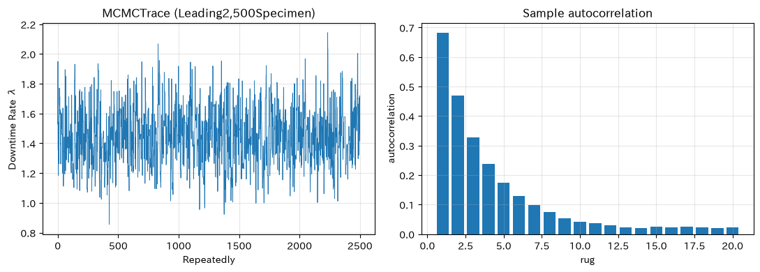
That’s right. Except for burn-ins, check traces, autocorrelations, and Monte Carlo standard errors.

Check with Python

def log_target_z(z):
    return ga_post * z - gb_post * np.exp(z)

mcmc_rng = np.random.default_rng(SEED + 74)
n_iter, burn = 16000, 3000
z = np.log(lambda_mean)
z_trace = np.empty(n_iter)
accepted = 0
for i in range(n_iter):
    proposal = z + mcmc_rng.normal(0, 0.22)
    if np.log(mcmc_rng.random()) < log_target_z(proposal) - log_target_z(z):
        z = proposal
        accepted += 1
    z_trace[i] = z

lambda_trace = np.exp(z_trace[burn:])
def autocorr(x, max_lag=40):
    centered = x - x.mean()
    ac = np.correlate(centered, centered, mode="full")[len(x)-1:len(x)+max_lag]
    return ac / ac[0]

acf = autocorr(lambda_trace)
positive_acf = acf[1:][acf[1:] > 0]
ess_approx = len(lambda_trace) / (1 + 2 * positive_acf.sum())
mcmc_summary = pd.DataFrame({
    "indicator": ["acceptance rate", "MCMCaverage", "Analytical Post-Hiad Average", "MCMC 2.5%", "MCMC 97.5%", "EstimateESS", "MCstandard error"],
    "value": [accepted/n_iter, lambda_trace.mean(), lambda_mean,
           *np.quantile(lambda_trace, [0.025, 0.975]), ess_approx,
           lambda_trace.std(ddof=1)/np.sqrt(ess_approx)],
})
display(mcmc_summary)

fig, axes = plt.subplots(1, 2, figsize=(11, 4))
axes[0].plot(lambda_trace[:2500], linewidth=0.6)
axes[0].set_title("MCMCTrace (Leading2,500Specimen)")
axes[0].set_xlabel("Repeatedly")
axes[0].set_ylabel("Downtime Rate λ")
axes[0].grid(alpha=0.3)
axes[1].bar(np.arange(1, 21), acf[1:21])
axes[1].set_title("Sample autocorrelation")
axes[1].set_xlabel("rug")
axes[1].set_ylabel("autocorrelation")
axes[1].grid(alpha=0.3)
plt.tight_layout()
plt.show()

	indicator	value
0	acceptance rate	0.5665
1	MCMCaverage	1.4504
2	Analytical Post-Hiad Average	1.4521
3	MCMC 2.5%	1.0835
4	MCMC 97.5%	1.8838
5	EstimateESS	2044.2499
6	MCstandard error	0.0045

Reading the results

The closeness between the MCMC mean and the analytic posterior mean is due to the implementation check in this example. Even with a large sample size, if there is autocorrelation among consecutive samples, the amount of independent information is low, and ESS is lower than the total sample size. In practice, multiple chains, $\hat R$, ESS, traces, divergence, and initial value sensitivity are checked, and the Monte Carlo error is sufficiently small than the accuracy required for the business before reporting probabilities.

No.075: Metropolis-Hastings — Diagnosing Proposal Breadth and Acceptance Rate

Meaning in Practice

The Metropolis-Hastings (MH) method is the fundamental MCMC technique that proposes candidates based on current values and determines adoption based on posterior probability ratios. If the proposal is too narrow, even if it is almost accepted, exploration slows down; if it is too large, rejections increase and the chain of action stops.

Approach to Analysis and Modeling

To always keep the nonconformance rate between 0 and 1, use symmetrical formal proposals on the $z=\mathrm{logit}(p)$. The logarithmic target density combining the beta posterior distribution and the Jacobian is

$$\log p(z\mid y)=a_{post}\log p+b_{post}\log(1-p)+C,\quad p=\mathrm{logit}^{-1}(z)$$

That’s right. We compare the range of multiple proposals and check not only the acceptance rate but also the error from ESS and the analysis solution.

Check with Python

def mh_beta(proposal_sd, seed, n_iter=12000, burn=2000):
    local_rng = np.random.default_rng(seed)
    z = np.log((a_post/(a_post+b_post)) / (1-a_post/(a_post+b_post)))
    out = np.empty(n_iter)
    accepted = 0
    def log_target(logit_p):
        p = expit(logit_p)
        return a_post*np.log(p) + b_post*np.log1p(-p)
    for i in range(n_iter):
        prop = z + local_rng.normal(0, proposal_sd)
        if np.log(local_rng.random()) < log_target(prop) - log_target(z):
            z = prop
            accepted += 1
        out[i] = expit(z)
    sample = out[burn:]
    ac = autocorr(sample, 100)
    pos = ac[1:][ac[1:] > 0]
    ess = len(sample)/(1+2*pos.sum())
    return sample, accepted/n_iter, ess

mh_rows = []
mh_samples = {}
for j, proposal_sd in enumerate([0.05, 0.35, 2.0]):
    sample, acc, ess = mh_beta(proposal_sd, SEED + 750 + j)
    mh_samples[proposal_sd] = sample
    mh_rows.append({"Proposal Width": proposal_sd, "acceptance rate": acc, "Post-event average": sample.mean(),
                    "Differences from analytical solutions": sample.mean()-a_post/(a_post+b_post), "EstimateESS": ess})
mh_df = pd.DataFrame(mh_rows)
display(mh_df)

for proposal_sd, sample in mh_samples.items():
    plt.plot(sample[:1000], linewidth=0.7, label=f"Proposal Width={proposal_sd}")
plt.title("By proposal widthMetropolis-HastingsDifferences in chain links")
plt.xlabel("Repeatedly")
plt.ylabel("nonconformity rate p")
plt.grid(alpha=0.3)
plt.legend()
plt.tight_layout()
plt.show()

	Proposal Width	acceptance rate	Post-event average	Differences from analytical solutions	EstimateESS
0	0.05	0.9097	0.0406	-0.0003	138.5534
1	0.35	0.5183	0.0412	0.0003	1814.6552
2	2.00	0.1148	0.0408	-0.0001	845.5656

Reading the results

Even if the acceptance rate is low, proposals with a small range only move gradually, and the ESS does not grow. A larger proposal width increases the number of intervals where the value remains the same. The intermediate width is efficient in this example, but there is no universal acceptance rate; it varies depending on dimension and target distribution. Acceptance rate alone is not a KPI; instead, ESS/sec, multi-chain matching, and Monte Carlo error for estimation are managed together.

No.076: Gibbs Sampling — Alternating between average and variation in filling times

Meaning in Practice

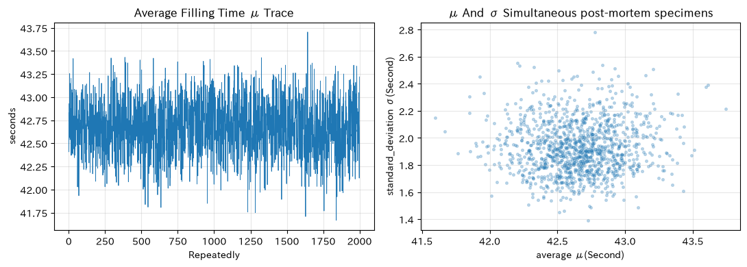
Both the process center $\mu$ and accuracy $\tau=1/\sigma^2$ of filling time are unknown. If you can sample directly from the conditional distribution of the other by fixing one, you can alternate updates with Gibbs Sampling.

Approach to Analysis and Modeling

$x_i\sim\mathcal N(\mu,\tau^{-1})$, a conjugate Normal-Gamma prior distribution

$$\mu\mid\tau\sim\mathcal N\left(\mu_0,(\kappa_0\tau)^{-1}\right),\qquad \tau\sim\mathrm{Gamma}(a_0,b_0)$$

Place. Alternate $\mu\mid\tau,x$ and $\tau\mid\mu,x$. Assuming independent normal data without chronological drift is confirmed in practice using control charts and residuals.

Check with Python

gibbs_rng = np.random.default_rng(SEED + 76)
mu0, kappa0, shape0, rate0 = 42.0, 0.5, 2.0, 4.0
n = len(fill_time)
n_gibbs, gibbs_burn = 14000, 2000
mu, tau = fill_time.mean(), 1/fill_time.var()
mu_chain = np.empty(n_gibbs)
sigma_chain = np.empty(n_gibbs)

for i in range(n_gibbs):
    # tau | mu, x
    shape = shape0 + (n + 1)/2
    rate = rate0 + 0.5*np.sum((fill_time-mu)**2) + 0.5*kappa0*(mu-mu0)**2
    tau = gibbs_rng.gamma(shape, 1/rate)
    # mu | tau, x
    kappa_n = kappa0 + n
    mu_n = (kappa0*mu0 + n*fill_time.mean())/kappa_n
    mu = gibbs_rng.normal(mu_n, np.sqrt(1/(kappa_n*tau)))
    mu_chain[i] = mu
    sigma_chain[i] = 1/np.sqrt(tau)

mu_sample = mu_chain[gibbs_burn:]
sigma_sample = sigma_chain[gibbs_burn:]
display(pd.DataFrame({
    "Estimated Subject": ["Average Filling Time μ", "standard_deviation σ"],
    "Post-event average": [mu_sample.mean(), sigma_sample.mean()],
    "95%lower_limit": [np.quantile(mu_sample, .025), np.quantile(sigma_sample, .025)],
    "95%upper": [np.quantile(mu_sample, .975), np.quantile(sigma_sample, .975)],
}))

fig, axes = plt.subplots(1, 2, figsize=(11, 4))
axes[0].plot(mu_sample[:2000], linewidth=0.6)
axes[0].set_title("Average Filling Time μ Trace")
axes[0].set_xlabel("Repeatedly")
axes[0].set_ylabel("seconds")
axes[0].grid(alpha=0.3)
axes[1].scatter(mu_sample[::10], sigma_sample[::10], s=7, alpha=0.25)
axes[1].set_title("μ And σ Simultaneous post-mortem specimens")
axes[1].set_xlabel("average μ(Second)")
axes[1].set_ylabel("standard_deviation σ(Second)")
axes[1].grid(alpha=0.3)
plt.tight_layout()
plt.show()

	Estimated Subject	Post-event average	95%lower_limit	95%upper
0	Average Filling Time μ	42.6703	42.0901	43.2449
1	standard_deviation σ	1.9306	1.5955	2.3738

Reading the results

Since the mean and standard deviation are kept as simultaneous distributions rather than fixed values, it is possible to separate and evaluate the possibility of “an increased mean” from a “possibility of increased variation.” Even with the Gibbs method, the specimen is not independent, so diagnosis is necessary. Also, the standard deviation of a standard model does not automatically separate short-term fluctuations from long-term drifts. Record time, equipment, and product types, and expand to hierarchical or chronological models as needed.

No.077: Introduction to PyMC — Declare Models and Estimate Nonconformance Rates

Meaning in Practice

In PyMC, the relationship between random variables and observations is declared as a model, and posterior distributions can be calculated using MCMC such as NUTS. A key advantage is that it is easy to gradually extend to models that include non-conjugate regression, hierarchical structures, and measurement errors.

Approach to Analysis and Modeling

First, $p\sim\mathrm{Beta}(1,1)$ like No.071, $k\sim\mathrm{Binomial}(n,p)$, is represented in PyMC. By starting with a simple model that can be matched with known analytical solutions, we verify library settings, random numbers, and summarization methods. target_accept is a value that adjusts the acceptance of proposals and is not an indicator of model validity.

Check with Python

with pm.Model() as defect_model:
    p = pm.Beta("p", alpha=a0, beta=b0)
    observed = pm.Binomial("observed", n=n_total, p=p, observed=k_total)
    idata = pm.sample(
        draws=1000, tune=1000, chains=2, cores=1,
        random_seed=SEED + 77,
        target_accept=0.9, progressbar=False,
        compute_convergence_checks=True,
    )

pymc_sample = idata.posterior["p"].values.reshape(-1)
pymc_summary = pm.stats.summary(idata, var_names=["p"], kind="all", round_to=5)
display(pymc_summary)
print(f"Analytic Post-Hidharma Average: {a_post/(a_post+b_post):.5f}")
print(f"PyMCPost-event average  : {pymc_sample.mean():.5f}")

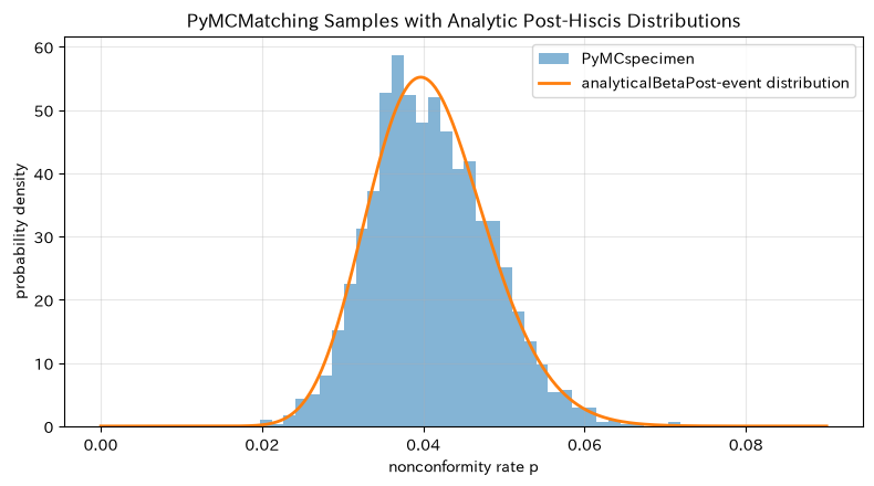
plt.hist(pymc_sample, bins=35, density=True, alpha=0.55, label="PyMCspecimen")
plt.plot(x, stats.beta.pdf(x, a_post, b_post), linewidth=2, label="analyticalBetaPost-event distribution")
plt.title("PyMCMatching Samples with Analytic Post-Hiscis Distributions")
plt.xlabel("nonconformity rate p")
plt.ylabel("probability density")
plt.grid(alpha=0.3)
plt.legend()
plt.tight_layout()
plt.show()

Initializing NUTS using jitter+adapt_diag...


Sequential sampling (2 chains in 1 job)


NUTS: [p]


Sampling 2 chains for 1_000 tune and 1_000 draw iterations (2_000 + 2_000 draws total) took 1 seconds.


We recommend running at least 4 chains for robust computation of convergence diagnostics

	mean	sd	hdi_3%	hdi_97%	mcse_mean	mcse_sd	ess_bulk	ess_tail	r_hat
p	0.041	0.0073	0.0282	0.0549	0.0003	0.0001	736.415	1017.243	1.0014

Post-analysis average: 0.04093
PyMC post-event average: 0.04103

Reading the results

If the post-poster mean of PyMC and the analysis solution are close to the Monte Carlo margin of error, and the histogram overlaps, the basic implementation can be checked. Check whether r_hat is close to 1 and whether ess_bulk and ess_tail are sufficient. In production, it is necessary to store model code, data versions, PyMC versions, seeds, chain counts, and diagnostic values, and not distribute only results without distributing warnings or divergence.

No.078: Hierarchical Bayes — Partially pooling factory-specific nonconformance rates

Meaning in Practice

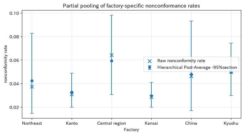
When ranking nonconformity rates by factory by raw ratio, factories with fewer inspections tend to have 0% or higher rates, mistaking chance for a difference in ability. Hierarchical Bayes retains information about each factory while borrowing information from a distribution common to all factories.

Approach to Analysis and Modeling

About the Factory $j$

$$k_j\sim\mathrm{Binomial}(n_j,p_j),\qquad p_j\sim\mathrm{Beta}(m\kappa,(1-m)\kappa)$$

Let’s say so. $m$ is the overall level, and $\kappa$ is the similarity between factories. Here, the predistribution is placed on the $(m,\kappa)$ grid, and weights are calculated based on the marginal likelihood of beta binomials, so instead of using only fixed hyperparameters, empirical Bayes are not used; their uncertainty is also reflected in the posterior distribution.

Check with Python

m_grid = np.linspace(0.008, 0.10, 90)
kappa_grid = np.geomspace(4, 180, 80)
M, KAPPA = np.meshgrid(m_grid, kappa_grid, indexing="ij")
ALPHA = M*KAPPA
BETA = (1-M)*KAPPA

log_weight = -KAPPA/60  # Loose preliminary index distribution in Kappa
for kj, nj in zip(plant_k, plant_n):
    log_weight += betaln(ALPHA+kj, BETA+nj-kj) - betaln(ALPHA, BETA)
log_weight -= log_weight.max()
weight = np.exp(log_weight)
weight /= weight.sum()

flat_rng = np.random.default_rng(SEED + 78)
grid_indices = flat_rng.choice(weight.size, size=12000, p=weight.ravel())
alpha_draw = ALPHA.ravel()[grid_indices]
beta_draw = BETA.ravel()[grid_indices]
hier_draws = np.column_stack([
    flat_rng.beta(alpha_draw+kj, beta_draw+nj-kj)
    for kj, nj in zip(plant_k, plant_n)
])

plant_df = pd.DataFrame({
    "Factory": plant_names,
    "number_of_inspections": plant_n,
    "non_conforming_number": plant_k,
    "Raw nonconformity rate": plant_k/plant_n,
    "Hierarchical Post-Hierarchy Average": hier_draws.mean(axis=0),
    "95%lower_limit": np.quantile(hier_draws, .025, axis=0),
    "95%upper": np.quantile(hier_draws, .975, axis=0),
})
display(plant_df)

pos = np.arange(len(plant_names))
plt.scatter(pos, plant_df["Raw nonconformity rate"], marker="x", s=70, label="Raw nonconformity rate")
plt.errorbar(pos, plant_df["Hierarchical Post-Hierarchy Average"],
             yerr=[plant_df["Hierarchical Post-Hierarchy Average"]-plant_df["95%lower_limit"],
                   plant_df["95%upper"]-plant_df["Hierarchical Post-Hierarchy Average"]],
             fmt="o", capsize=4, label="Hierarchical Post-Average -95%section")
plt.xticks(pos, plant_names)
plt.title("Partial pooling of factory-specific nonconformance rates")
plt.xlabel("Factory")
plt.ylabel("nonconformity rate")
plt.grid(alpha=0.3)
plt.legend()
plt.tight_layout()
plt.show()

	Factory	number_of_inspections	non_conforming_number	Raw nonconformity rate	Hierarchical Post-Hierarchy Average	95%lower_limit	95%upper
0	Northeast	80	3	0.0375	0.0425	0.0148	0.0828
1	Kanto	520	16	0.0308	0.0327	0.0198	0.0489
2	Central region	140	9	0.0643	0.0593	0.0305	0.0982
3	Kansai	950	27	0.0284	0.0297	0.0199	0.0411
4	China	65	3	0.0462	0.0479	0.0171	0.0934
5	Kyushu	300	15	0.0500	0.0497	0.0298	0.0745

Reading the results

Factories with fewer inspections tend to reduce the overall inspection level more strongly and have wider sections. This is not a process to eliminate factory differences, but rather partial pooling that handles the extreme values of a small number of data with uncertainty tolerance. We do not directly link the reduced rankings to personnel evaluations, but instead verify comparability in terms of material composition, product difficulty, and measurement standards. Factories with processes so different that a common distribution cannot be established, they need to be divided into separate groups.

No.079: Bayesian Prediction Distribution — Predicting the Number of Nonconformities in the Next Inspection

Meaning in Practice

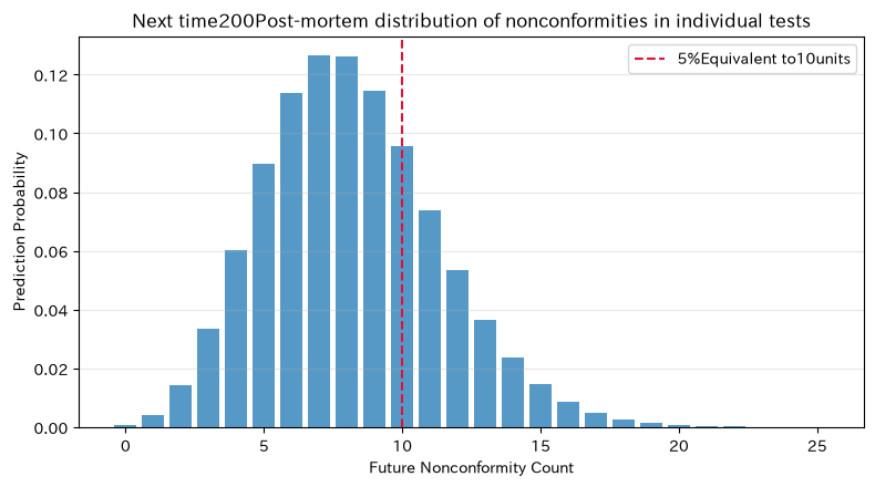
Quality assurance wants to know not only the true nonconformity rate, but also “how many nonconformities will appear in the next 200 units” and “what is the risk of the rate of the rate dropping above 5%.” Predicted distributions include both parameter uncertainty and future random variations.

Approach to Analysis and Modeling

Under posterior distribution $p\mid y\sim\mathrm{Beta}(a,b)$, the future $m$ nonconformities $\tilde k$ are the beta binomial distribution.

$$p(\tilde k\mid y)=\binom{m}{\tilde k} \frac{B(a+\tilde k,b+m-\tilde k)}{B(a,b)}$$

We will follow the rules. $p$ is wider than the binomial distribution fixed to the posterior mean, allowing the uncertainty of the estimate to be reflected in the plan.

Check with Python

future_n = 200
future_k = np.arange(future_n+1)
pred_pmf = stats.betabinom.pmf(future_k, future_n, a_post, b_post)
pred_interval = stats.betabinom.ppf([0.025, 0.975], future_n, a_post, b_post).astype(int)
risk_5pct = stats.betabinom.sf(9, future_n, a_post, b_post)  # 10 or more

display(pd.DataFrame({
    "indicator": ["Number of Upcoming Examinations", "Average number of forecast mismatches", "95%Lower Limit of Forecast Section", "95%Forecast Section Upper Limit", "P(10more than several = 5%That's all.)"],
    "value": [future_n, future_n*a_post/(a_post+b_post), *pred_interval, risk_5pct],
}))

show = future_k <= 25
plt.bar(future_k[show], pred_pmf[show], alpha=0.75)
plt.axvline(10, color="crimson", linestyle="--", label="5%Equivalent to10units")
plt.title("Next time200Post-mortem distribution of nonconformities in individual tests")
plt.xlabel("Future Nonconformity Count")
plt.ylabel("Prediction Probability")
plt.grid(axis="y", alpha=0.3)
plt.legend()
plt.tight_layout()
plt.show()

	indicator	value
0	Number of Upcoming Examinations	200.0000
1	Average number of forecast mismatches	8.1855
2	95%Lower Limit of Forecast Section	3.0000
3	95%Forecast Section Upper Limit	15.0000
4	P(10more than several = 5%That's all.)	0.3164

Reading the results

By looking not only at the forecast average but also within the 95% forecast interval, you can understand the possible swings during the next inspection. A probability of 5% or higher is a criterion for preparing additional testing personnel or isolation spaces. The credit range is within the range of unknown rates $p$, while the forecast range is the range of future non-conformities, with different uses. The validity of forecasts is continuously verified with subsequent comparisons against actual results.

No.080: Bayesian A/B Test — Determining the Deployment of New Cleaning Conditions

Meaning in Practice

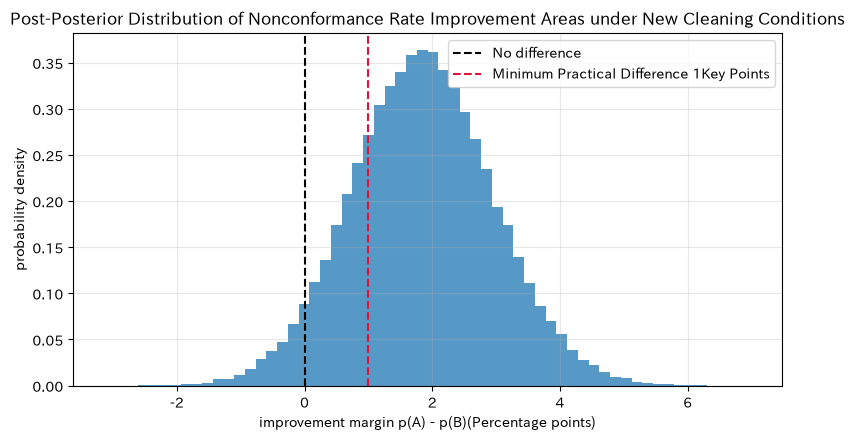
When comparing the current Condition A and the new Cleanup Condition B, evaluate not only the “difference” but also the probability that B will outperform A, the probability that the improvement will meet investment criteria, and the loss if misdeployed. This allows us to distinguish between statistical differences and those that are meaningful for business purposes.

Approach to Analysis and Modeling

By placing an independent $\mathrm{Beta}(1,1)$ prior distribution for the nonconformity rates of both conditions, each posterior distribution can be analytically obtained. From the post-event sample, the difference $\Delta=p_A-p_B$ is calculated, and $P(\Delta>0)$ and $P(\Delta>0.01)$ for the minimum practical deviation of 1 point are obtained. In actual A/B, variety, material lots, equipment, and duration are randomized or adjusted to avoid confusion.

Check with Python

ab_rng = np.random.default_rng(SEED + 80)
draws = 100000
p_a = ab_rng.beta(1+ab_k["Current Conditions"], 1+ab_n["Current Conditions"]-ab_k["Current Conditions"], draws)
p_b = ab_rng.beta(1+ab_k["New Cleaning Conditions"], 1+ab_n["New Cleaning Conditions"]-ab_k["New Cleaning Conditions"], draws)
delta = p_a - p_b

ab_table = pd.DataFrame({
    "condition": ["Current ConditionsA", "New Cleaning ConditionsB"],
    "number_of_inspections": [ab_n["Current Conditions"], ab_n["New Cleaning Conditions"]],
    "non_conforming_number": [ab_k["Current Conditions"], ab_k["New Cleaning Conditions"]],
    "Observation mismatch rate": [ab_k["Current Conditions"]/ab_n["Current Conditions"], ab_k["New Cleaning Conditions"]/ab_n["New Cleaning Conditions"]],
    "Post-event average": [p_a.mean(), p_b.mean()],
})
display(ab_table)
display(pd.DataFrame({
    "judgment indicator": ["P(BbutAlower)", "P(The range of improvement1Over Points)", "Post-Mortem Average of Improvement Margins", "improvement range95%credit range"],
    "value": [f"{np.mean(delta>0):.3%}", f"{np.mean(delta>0.01):.3%}",
           f"{delta.mean():.3%}", f"{np.quantile(delta,.025):.3%} 〜 {np.quantile(delta,.975):.3%}"],
}))

plt.hist(delta*100, bins=60, density=True, alpha=0.75)
plt.axvline(0, color="black", linestyle="--", label="No difference")
plt.axvline(1, color="crimson", linestyle="--", label="Minimum Practical Difference 1Key Points")
plt.title("Post-Posterior Distribution of Nonconformance Rate Improvement Areas under New Cleaning Conditions")
plt.xlabel("improvement margin p(A) - p(B)(Percentage points)")
plt.ylabel("probability density")
plt.grid(alpha=0.3)
plt.legend()
plt.tight_layout()
plt.show()

	condition	number_of_inspections	non_conforming_number	Observation mismatch rate	Post-event average
0	Current ConditionsA	650	32	0.0492	0.0507
1	New Cleaning ConditionsB	620	19	0.0306	0.0322

	judgment indicator	value
0	P(BbutAlower)	95.283%
1	P(The range of improvement1Over Points)	77.666%
2	Post-Mortem Average of Improvement Margins	1.847%
3	improvement range95%credit range	-0.316% 〜 4.062%

Reading the results

The probability that B is lower than A and the probability of improving by more than one point are different. If the former is higher but the latter does not meet investment standards, additional testing rather than full rollout may be appropriate. In the final decision, runoff losses, change costs, and side effects on takt and other quality characteristics are included in the loss function. It is important not to change the probability threshold after seeing the results, and to agree on decision-making rules before the exam.

Practical Implications Seen Through Target Exercise

1. Report by probability, not by dots: Setting post-mortem averages, credit intervals, and the probability of exceeding standards concretely clarifies discussions about additional inspections, suspensions, and deployments.
2. Making pre-distribution auditable: Record how many weights were used for past data, similar processes, and expert judgments.
3. Distinguishing between forecasting and parameter estimation: Future counts include both uncertainty in process rates and future unexpected fluctuations.
4. Don’t overrank a minority: Information is shared between factories in a hierarchical bay, showing reductions and intervals based on the number of inspections.
5. MCMCInclude diagnostics in deliverables: Not only acceptance rate, but also traces, multiple chains, $\hat R$, ESS, divergence, and MC error are stored.
6. Converting statistical differences into economic value: In addition to the superior probability of A/B, decisions are made using the minimum practical difference and loss function.

What is necessary for practical implementation

• Definition of decision-making: Decide in advance who will conduct additional inspections, stops, or deployments at what post-event and predictive probabilities.
• Verification of the Data Generation Process: Record equipment, molds, materials, varieties, shifts, inspectors, and time, and check interchangeability and independence.
• Governance of the prior distribution: Review the basis, update date, scope, effective sample size, and sensitivity difference from the weak information prior distribution
• Model Verification: Postmortem checks, out-of-time validation, calibration, and cross-referencing with known simple models
• Managing Computational Quality: Save environment, dependency libraries, seeds, chains, diagnostic values, warnings, and execution logs
• Connection to operational losses: Quantify losses from missed opportunities, over-stopping, inspections, capital investments, and quality leaks, turning probability into action.
• Phased Implementation: Reproduce and verify with past data, proceed to shadow operations, trials in limited processes, standardization of work, and regular monitoring.

The Bayesian model is not a device that automatically corrects on-site judgments. Value is only created when data collection, process knowledge, model diagnostics, and decision-making responsibility are designed together.

Conclusion

From No.071 to No.080, we started with conjugate updates for Beta Bernoulli and Gamma Poissons, then implemented sequential updates, MCMC, Metropolis-Hastings, Gibbs Sampling, PyMC, hierarchical Bayes, post-prediction, and Bayesian A/B testing.

The core idea is to integrate past insights and observations under transparent rules, translating unknowns and uncertainties of future outcomes into probabilities that the field can judge. Operate in a state where you can clearly state the prior distribution, likelihood, model structure, computational diagnosis, and loss function, and explain which assumptions the results depend on.

Consultations for Corporations

At Mathematical Laboratory, we support everything from quality data analysis, Bayesian statistical models, hierarchical models, anomaly and failure prediction, experimental design, Python training, and PoC to operational implementation in manufacturing. You can consult with us at stages such as “wanting to utilize a small amount of data,” “determining nonconformance rates and downtime by probabilism,” “making inter-factory comparisons fair,” or “establishing model diagnostics and operational standards.”

📩 Contact Us: surikobo.co.jp/contact Please feel free to consult us first.