Predicting quality, stoppages, and man-hours from process conditions: 10 exercises on the manufacturing regression model

In manufacturing sites, factors such as temperature, processing speed, vibration, material condition, and maintenance days all simultaneously affect energy intensity, nonconformities, slight stops, and recovery man-hours. In this article, we will implement Linear regression,Ridge、Lasso、ElasticNetlogistic regression, Poisson regression, negative binomial regression,GLM、GAM, quantile regression based on the production performance of a fictional precision parts factory.

The goal is not to memorize the model name, but to use a model that matches the nature of the target variable to judge “which conditions to apply,” “where to be wary of nonconformance risks,” and “how many person-hours to expect in cases worse than average.” The target is a probability and statistics Python implementation No.061〜No.070 with 100 Exercises.

[!NOTE] This material is a notebook previously used by Surikoubo (or personally by the representative, Kazuyama), and has been reconstructed, edited, and published with the company’s permission.
All data listed is fictional and has no relation whatsoever to real companies, factories, or figures.

Introduction: Practical Challenges in Manufacturing Covered in This Article

In a hypothetical precision parts factory, each production batch records process temperature, processing speed, equipment vibration, material moisture content, and days elapsed after maintenance. Managers need to answer the following questions to determine the standard conditions and staffing plan for the following month.

• What are the conditions to increase the power intensity?
• How to narrow down the variables needed for explanation from many similar sensor metrics
• Is it acceptable to treat the presence or absence of nonconformity and the number of slight stops in the same regression?
• How to represent the risk when the variation in microstops is greater than average?
• How to estimate not only average recovery time but also cases that take longer periods

A regression model is a tool that quantifies the relationship between results and factors and makes predictions when conditions change. However, the appropriate distribution and link function differ depending on whether the target variable is a continuous quantity, 0/1, number of cases, or a positive distorted value.

Common situations on site

• Interpreting the coefficients of single regression as causal effects without confounding or confirming the scope of operations
• Highly correlated sensors are deployed simultaneously, and the coefficient codes change with each meeting.
• Predicting the mismatch rate using standard linear regression, resulting in values below 0% or over 100%.
• Treat the number of stopped events as a normal distribution and ignore the property of integers greater than or equal to zero
• Selecting models based solely on average forecast accuracy and overlooking upside during busy periods

In model selection, not only prediction accuracy but also the mechanism of data generation, coefficient stability, whether the purpose is explanatory or forecasting, and whether losses during decision-making are symmetrical are clarified.

Why is this issue so difficult to judge?

Let the general form of regression be given the mean structure.

$$g\{E(Y\mid X)\}=\beta_0+\beta_1x_1+\cdots+\beta_px_p$$

That’s what I write. $g$ is a link function. Identity links are typical for linear regression of continuous quantities, logit for binary data, and logarithmic links for number of cases. Even with the same explanatory variable, the distribution and links need to be adjusted to match the $Y$ scale.

Also, what is found in predictions is, in principle, related, not causal. Even if the temperature coefficient is positive, it does not necessarily mean that raising the temperature will necessarily worsen the condition. Considering variety, equipment, workers, chronological order, and rules for changing conditions, if you want to know the effects of the intervention, separately design experimental plans and causal inference.

Overview of Exercise covered this time

No.	Theme	Questions in the Manufacturing Industry
061	linear regression	Can you explain the power intensity from process conditions?
062	Ridge Return	Can the coefficient be stabilized even if there are correlated sensors?
063	Lasso Return	Can you narrow down variables with minimal impact from the candidates?
064	ElasticNet	Can variable selection and correlation variable retention be balanced?
065	Logistic Regression	Can the probability of batch mismatch be estimated from 0 to 1?
066	Poisson Return	Can the number of minor downtime be compared considering operating hours?
067	negative binomial regression	Can we factor in the overdispersion of the number of cases?
068	GLM	Can distorted recovery man-hours be represented by distribution and linkage?
069	GAM	Can nonlinear effects such as temperature be smoothly captured?
070	Quantile Regression	Can median recovery time and upside risk be separated and predicted?

No.061–064 deal with continuous quantities and regularization, No.065–068 deal with probability distributions according to the target variable, and No.069–070 deal with structures that cannot be represented by means or lines alone.

Preparing the Python environment

Generate fictional data with NumPy and create tables with pandas. scikit-learn is used for preprocessing, regularization, and predictive evaluation; statsmodels for statistical models; and matplotlib for visualization. japanize_matplotlib is used only for Japanese display purposes; seaborn or external data is not used. Fix the random number seed so that the same result can be reproduced.

import platform
import numpy as np
import pandas as pd
import scipy
import sklearn
from sklearn.compose import TransformedTargetRegressor
from sklearn.linear_model import LinearRegression, Ridge, Lasso, ElasticNet, LogisticRegression
from sklearn.metrics import mean_squared_error, roc_auc_score, log_loss
from sklearn.model_selection import train_test_split
from sklearn.pipeline import make_pipeline
from sklearn.preprocessing import StandardScaler, SplineTransformer
import statsmodels.api as sm
import matplotlib
import matplotlib.pyplot as plt
import japanize_matplotlib

SEED = 20260711
rng = np.random.default_rng(SEED)
plt.rcParams["figure.figsize"] = (8, 4.5)
plt.rcParams["axes.unicode_minus"] = False

print(f"Python      : {platform.python_version()}")
print(f"NumPy       : {np.__version__}")
print(f"pandas      : {pd.__version__}")
print(f"SciPy       : {scipy.__version__}")
print(f"scikit-learn: {sklearn.__version__}")
print(f"statsmodels : {sm.__version__}")
print(f"Matplotlib  : {matplotlib.__version__}")
print(f"random seed : {SEED}")

Python      : 3.13.1
NumPy       : 2.5.1
pandas      : 3.0.3
SciPy       : 1.18.0
scikit-learn: 1.9.0
statsmodels : 0.14.6
Matplotlib  : 3.11.0
random seed : 20260711

Creation of Fictional Data

Generate production performance for 420 batches. cooling_flow is the cooling flow rate strongly correlated with process temperature, and sensor_temp_2 is a redundant separate sensor for temperature. These reproduce situations where regularization is necessary.

The number of slight stops is generated using a gamma-Poisson mixture, varying due to batch-specific invisible difficulties. Therefore, the variance is larger than the mean, allowing us to later observe the difference between Poisson regression and negative binomial regression. Model training does not use generative formulas or true coefficients.

n = 420
temperature = rng.normal(72, 4.2, n)
speed = rng.normal(118, 13, n)
vibration = np.clip(rng.gamma(3.2, 0.32, n), 0.15, None)
moisture = rng.normal(0.82, 0.16, n)
maintenance_days = rng.integers(1, 121, n)
operating_hours = rng.uniform(5.5, 10.0, n)
cooling_flow = 34 - 0.32 * temperature + rng.normal(0, 0.9, n)
sensor_temp_2 = temperature + rng.normal(0, 0.7, n)
ambient_humidity = rng.normal(56, 9, n)

energy = (31 + 0.34 * speed + 0.75 * (temperature - 72)
          + 2.8 * vibration + rng.normal(0, 3.2, n))
defect_logit = (-3.1 + 0.15 * (temperature - 72) + 0.62 * (vibration - 1)
                + 0.018 * maintenance_days + 0.55 * (moisture - 0.82))
defect = rng.binomial(1, 1 / (1 + np.exp(-defect_logit)))
stop_rate = np.exp(-2.0 + 0.42 * vibration + 0.009 * maintenance_days)
latent_rate = rng.gamma(shape=1.5, scale=stop_rate / 1.5)
micro_stops = rng.poisson(operating_hours * latent_rate)
recovery_hours = rng.gamma(
    shape=2.5,
    scale=np.exp(-1.25 + 0.012 * maintenance_days + 0.27 * vibration) / 2.5,
)
cycle_time = (41 + 0.15 * speed + 4.6 * vibration + 0.020 * maintenance_days
              + rng.normal(0, 1.5 + 1.3 * vibration, n))
quality_loss = (1.8 + 0.12 * (temperature - 72) ** 2
                + 0.015 * (speed - 118) ** 2 + 1.7 * vibration + rng.normal(0, 1.2, n))

df = pd.DataFrame({
    "temperature": temperature, "sensor_temp_2": sensor_temp_2, "speed": speed,
    "vibration": vibration, "moisture": moisture, "maintenance_days": maintenance_days,
    "operating_hours": operating_hours, "cooling_flow": cooling_flow,
    "ambient_humidity": ambient_humidity, "energy": energy, "defect": defect,
    "micro_stops": micro_stops, "recovery_hours": recovery_hours,
    "cycle_time": cycle_time, "quality_loss": quality_loss,
})

display(df.head().round(3))
display(pd.DataFrame({
    "indicator": ["batch quantity", "nonconformity rate", "Mean of microstops", "Dispersion of micro-stopping", "Average Recovery Workload"],
    "value": [len(df), df.defect.mean(), df.micro_stops.mean(),
           df.micro_stops.var(), df.recovery_hours.mean()],
}).round(3))

	temperature	sensor_temp_2	speed	vibration	moisture	maintenance_days	operating_hours	cooling_flow	ambient_humidity	energy	defect	micro_stops	recovery_hours	cycle_time	quality_loss
0	66.740	66.167	126.618	1.062	0.989	10	7.704	11.849	61.413	71.472	0	2	0.442	60.080	7.476
1	70.616	70.193	135.361	0.377	1.015	89	9.550	11.421	51.120	75.155	0	3	0.609	64.640	7.523
2	73.686	73.601	107.679	1.341	0.570	43	6.338	10.085	76.765	73.063	0	0	0.488	65.133	6.173
3	69.063	68.940	124.009	0.150	0.690	120	8.677	12.773	41.372	73.693	1	2	3.237	62.716	4.116
4	66.060	65.541	108.298	1.641	1.132	68	6.988	12.005	44.895	65.630	0	2	1.241	70.649	10.696

	indicator	value
0	batch quantity	420.000
1	nonconformity rate	0.143
2	Mean of microstops	3.133
3	Dispersion of micro-stopping	10.946
4	Average Recovery Workload	0.811

No.061: Linear Regression — Explaining Power Intensity from Process Conditions

Meaning in Practice

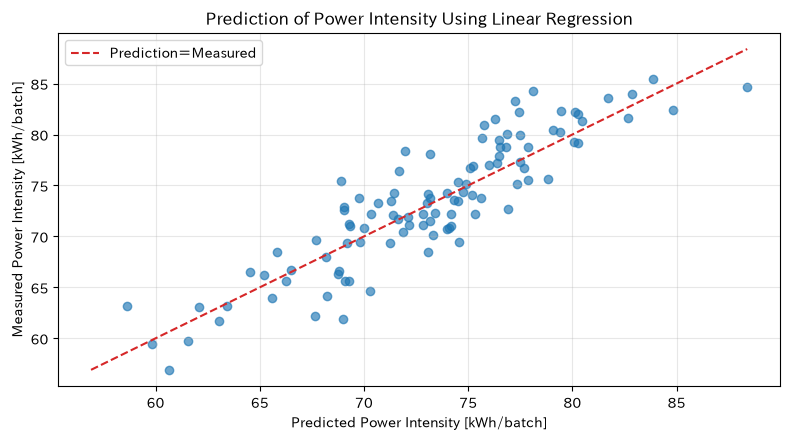
By quantifying the relationship between power intensity and process conditions, hypotheses about potential for energy savings through setting changes can be created. Linear regression is easy to explain and useful as a reference model.

Approach to Analysis and Modeling

Linear regression is

$$y_i=\beta_0+\sum_{j=1}^{p}\beta_jx_{ij}+\varepsilon_i$$

and minimize the sum of squares of the residual $\sum_i(y_i-\hat y_i)^2$. Coefficient $\beta_j$ is “the average change of $x_j$ 1 unit increase when other variables are constant.” Separate training and evaluation data, and verify with RMSE on unknown data.

Check with Python

reg_features = ["temperature", "speed", "vibration", "maintenance_days"]
X_train, X_test, y_train, y_test = train_test_split(
    df[reg_features], df["energy"], test_size=0.25, random_state=SEED
)
ols = LinearRegression().fit(X_train, y_train)
ols_pred = ols.predict(X_test)

ols_result = pd.DataFrame({"Explanatory variable": reg_features, "coefficient": ols.coef_})
display(ols_result.round(3))
print(f"slice      : {ols.intercept_:.3f}")
print(f"ReceptionRMSE  : {mean_squared_error(y_test, ols_pred)**0.5:.3f}")

plt.scatter(ols_pred, y_test, alpha=0.65)
limits = [min(ols_pred.min(), y_test.min()), max(ols_pred.max(), y_test.max())]
plt.plot(limits, limits, "--", color="tab:red", label="Prediction＝Measured")
plt.title("Prediction of Power Intensity Using Linear Regression")
plt.xlabel("Predicted Power Intensity [kWh/batch]")
plt.ylabel("Measured Power Intensity [kWh/batch]")
plt.grid(True, alpha=0.3)
plt.legend()
plt.tight_layout()
plt.show()

	Explanatory variable	coefficient
0	temperature	0.695
1	speed	0.353
2	vibration	2.979
3	maintenance_days	0.005

Slices: -21.146
Rating RMSE: 2.856

Reading the results

Evaluation RMSE shows typical forecast errors for unknown batches in original units. Since the magnitude of the coefficient depends on the unit, temperature and maintenance period values cannot be used directly for importance comparison. Also, if the relationship between prediction and actual measurement systematically deviates from the straight line, consider nonlinear terms, interactions, and unobserved factors. Coefficients are conditional relationships within the scope of operation and do not guarantee causal effects from changes in settings.

No.062: Ridge Regression — Stabilizing Coefficients of Correlated Sensors

Meaning in Practice

When sensors measuring the same phenomenon or controlled linked settings are used simultaneously, multicollinearity can make the coefficients unstable. Even if the predicted values are similar, if the coefficient signs or sizes change due to sample differences, it becomes difficult to use for explaining improvement measures.

Approach to Analysis and Modeling

Ridge regression adds the L2 penalty to the standardized coefficient,

$$\min_{\beta}\left\{\sum_i(y_i-\beta_0-x_i^T\beta)^2+\alpha\sum_j\beta_j^2\right\}$$

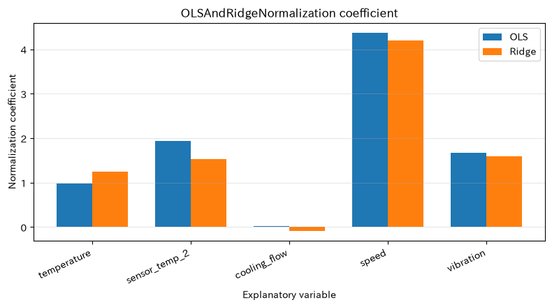
Solve it. The larger the $\alpha$, the smaller the coefficient shrinks toward zero, but usually it is not strictly zero. By exchanging bias and reduced variance due to shrinkage, the goal is to stabilize forecasts and coefficients.

Check with Python

corr_features = ["temperature", "sensor_temp_2", "cooling_flow", "speed", "vibration"]
Xr_train, Xr_test, yr_train, yr_test = train_test_split(
    df[corr_features], df["energy"], test_size=0.25, random_state=SEED
)
scaler = StandardScaler().fit(Xr_train)
Xr_train_z, Xr_test_z = scaler.transform(Xr_train), scaler.transform(Xr_test)

ols_z = LinearRegression().fit(Xr_train_z, yr_train)
ridge = Ridge(alpha=12).fit(Xr_train_z, yr_train)
ridge_comparison = pd.DataFrame({
    "Explanatory variable": corr_features, "OLSNormalization coefficient": ols_z.coef_, "RidgeNormalization coefficient": ridge.coef_,
})
display(ridge_comparison.round(3))
print(f"OLSReceptionRMSE   : {mean_squared_error(yr_test, ols_z.predict(Xr_test_z))**0.5:.3f}")
print(f"RidgeReceptionRMSE : {mean_squared_error(yr_test, ridge.predict(Xr_test_z))**0.5:.3f}")

x = np.arange(len(corr_features))
plt.bar(x - 0.18, ols_z.coef_, width=0.36, label="OLS")
plt.bar(x + 0.18, ridge.coef_, width=0.36, label="Ridge")
plt.title("OLSAndRidgeNormalization coefficient")
plt.xlabel("Explanatory variable")
plt.ylabel("Normalization coefficient")
plt.xticks(x, corr_features, rotation=25, ha="right")
plt.grid(True, axis="y", alpha=0.3)
plt.legend()
plt.tight_layout()
plt.show()

	Explanatory variable	OLSNormalization coefficient	RidgeNormalization coefficient
0	temperature	0.981	1.252
1	sensor_temp_2	1.937	1.523
2	cooling_flow	0.024	-0.079
3	speed	4.368	4.201
4	vibration	1.663	1.597

OLS Rating RMSE: 2.880
Ridge Rating RMSE: 2.878

Reading the results

Temperature, separate temperature sensors, and cooling flow rate are correlated, making it easier for OLS to unstably distribute effects among variables. Ridge reduces the normalization factor and suppresses extreme coefficients for variables with similar information. If RMSE does not deteriorate significantly and the coefficient stabilizes, it is a promising monitoring model. However, contraction coefficients are not interpreted as physical laws or causal effects. $\alpha$ is decided by cross-verification during the actual test.

No.063: Lasso Regression — Narrowing down variables as candidates for improvement

Meaning in Practice

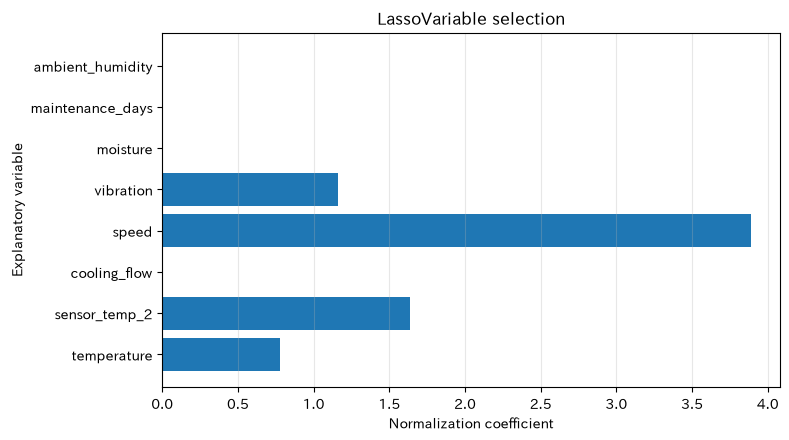
Even when collecting many sensors, the cost of maintaining them all at all times is not insignificant. Lasso can set unnecessary coefficients to zero, making it useful for narrowing down candidates needed for predictions and creating concise models.

Approach to Analysis and Modeling

Lasso uses L1 penalties,

$$\min_{\beta}\left\{\sum_i(y_i-\beta_0-x_i^T\beta)^2+\alpha\sum_j|\beta_j|\right\}$$

Solve it. Since the effect of penalties changes depending on the scale of variables, standardization is essential. In groups of highly correlated variables, only one may be arbitrarily retained, so the selection result is not considered the only physical cause.

Check with Python

wide_features = corr_features + ["moisture", "maintenance_days", "ambient_humidity"]
Xl_train, Xl_test, yl_train, yl_test = train_test_split(
    df[wide_features], df["energy"], test_size=0.25, random_state=SEED
)
lasso_pipe = make_pipeline(StandardScaler(), Lasso(alpha=0.45, max_iter=20000))
lasso_pipe.fit(Xl_train, yl_train)
lasso_coef = lasso_pipe.named_steps["lasso"].coef_
lasso_table = pd.DataFrame({
    "Explanatory variable": wide_features, "Normalization coefficient": lasso_coef,
    "Choice": np.where(np.abs(lasso_coef) > 1e-8, "Candidate for Employment", "0(Excluded candidate)"),
})
display(lasso_table.round(3))
print(f"ReceptionRMSE: {mean_squared_error(yl_test, lasso_pipe.predict(Xl_test))**0.5:.3f}")

plt.barh(wide_features, lasso_coef)
plt.title("LassoVariable selection")
plt.xlabel("Normalization coefficient")
plt.ylabel("Explanatory variable")
plt.grid(True, axis="x", alpha=0.3)
plt.tight_layout()
plt.show()

	Explanatory variable	Normalization coefficient	Choice
0	temperature	0.779	Candidate for Employment
1	sensor_temp_2	1.639	Candidate for Employment
2	cooling_flow	-0.000	0(Excluded candidate)
3	speed	3.886	Candidate for Employment
4	vibration	1.160	Candidate for Employment
5	moisture	0.000	0(Excluded candidate)
6	maintenance_days	0.000	0(Excluded candidate)
7	ambient_humidity	0.000	0(Excluded candidate)

RMSE rating: 3.013

Reading the results

Variables with zero coefficients are candidates with small additional predictive information under the current penalty intensity and the presence of other variables. This is not a conclusion that “it will not affect the process.” Since selection depends on the specimen and $\alpha$, the frequency of selection, maintenance costs, and measurement reliability in resampling are combined to avoid irreversible decisions such as sensor obsolescence.

No.064: ElasticNet — Balancing Selection and Correlation Variable Retention

Meaning in Practice

Manufacturing data contains a collection of correlated variables such as temperature sensor clusters and vibration frequency bands. ElasticNet is a good choice when you want to handle related variables collectively while maintaining the simplicity of Lasso.

Approach to Analysis and Modeling

ElasticNet combines L1 and L2,

$$\min_{\beta}\left\{\frac{1}{2n}\|y-X\beta\|_2^2+\alpha\left(\rho\|\beta\|_1+\frac{1-\rho}{2}\|\beta\|_2^2\right)\right\}$$

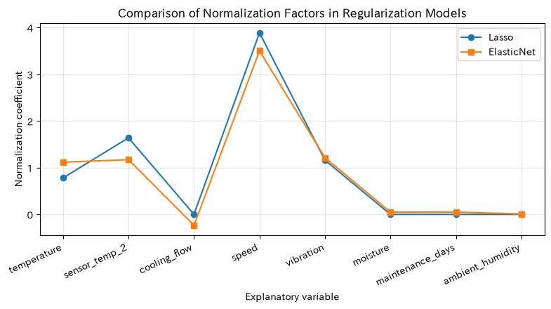
Solve it. $\rho=1$ is Lasso, and the closer you get to $\rho=0$, the more Ridge-like it gets. Here, we compare it with Lasso using the same learning and assessment split.

Check with Python

enet_pipe = make_pipeline(
    StandardScaler(), ElasticNet(alpha=0.35, l1_ratio=0.45, max_iter=20000)
)
enet_pipe.fit(Xl_train, yl_train)
enet_coef = enet_pipe.named_steps["elasticnet"].coef_
regularized_comparison = pd.DataFrame({
    "Explanatory variable": wide_features, "Lasso": lasso_coef, "ElasticNet": enet_coef,
})
display(regularized_comparison.round(3))

model_rmse = pd.DataFrame({
    "Model": ["Lasso", "ElasticNet"],
    "ReceptionRMSE": [
        mean_squared_error(yl_test, lasso_pipe.predict(Xl_test))**0.5,
        mean_squared_error(yl_test, enet_pipe.predict(Xl_test))**0.5,
    ],
})
display(model_rmse.round(3))

x = np.arange(len(wide_features))
plt.plot(x, lasso_coef, "o-", label="Lasso")
plt.plot(x, enet_coef, "s-", label="ElasticNet")
plt.title("Comparison of Normalization Factors in Regularization Models")
plt.xlabel("Explanatory variable")
plt.ylabel("Normalization coefficient")
plt.xticks(x, wide_features, rotation=25, ha="right")
plt.grid(True, alpha=0.3)
plt.legend()
plt.tight_layout()
plt.show()

	Explanatory variable	Lasso	ElasticNet
0	temperature	0.779	1.117
1	sensor_temp_2	1.639	1.171
2	cooling_flow	-0.000	-0.234
3	speed	3.886	3.501
4	vibration	1.160	1.214
5	moisture	0.000	0.049
6	maintenance_days	0.000	0.050
7	ambient_humidity	0.000	0.009

	Model	ReceptionRMSE
0	Lasso	3.013
1	ElasticNet	3.064

Reading the results

ElasticNet uses L2 components to easily divide correlated temperature system variable information into multiple coefficients and retain it. Although the number of variables can increase compared to Lasso, it can mitigate the instability of leaving only one correlation group. In practice, RMSE, coefficient reproducibility, measurement cost, and ease of explanation are evaluated as the criteria, and $\alpha$ and $\rho$ are selected through cross-validation.

No.065: Logistic Regression — Predicting the Probability of Batch Nonconformity

Meaning in Practice

If the objective variable is a binary of pass/fail, what is needed is not the continuous value itself but the probability of non-conformity. Missed and inspection costs can be linked to additional tests, such as redirecting batches exceeding the threshold probabilities.

Approach to Analysis and Modeling

Logistic regression

$$\log\frac{p_i}{1-p_i}=\beta_0+x_i^T\beta, \qquad p_i=P(Y_i=1\mid x_i)$$

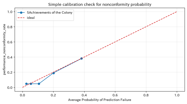
That’s how it is placed. $e^{\beta_j}$ is the odds ratio per unit increase with other variables constant. ROC-AUC ranks the results, while log loss evaluates the probability of the probability. The operational threshold is not fixed at 0.5, but is determined based on the costs of missed and over-inspections.

Check with Python

clf_features = ["temperature", "vibration", "moisture", "maintenance_days"]
Xc_train, Xc_test, yc_train, yc_test = train_test_split(
    df[clf_features], df["defect"], test_size=0.25, stratify=df["defect"], random_state=SEED
)
logit_pipe = make_pipeline(StandardScaler(), LogisticRegression(C=10, max_iter=5000))
logit_pipe.fit(Xc_train, yc_train)
prob = logit_pipe.predict_proba(Xc_test)[:, 1]
logit_coef = logit_pipe.named_steps["logisticregression"].coef_[0]
display(pd.DataFrame({
    "Explanatory variable": clf_features, "Normalization coefficient": logit_coef, "standard_deviation1Odds ratios for individual pieces": np.exp(logit_coef),
}).round(3))
print(f"nonconformity rate : {yc_test.mean():.3f}")
print(f"ROC-AUC  : {roc_auc_score(yc_test, prob):.3f}")
print(f"Log loss : {log_loss(yc_test, prob):.3f}")

bins = pd.qcut(prob, q=5, duplicates="drop")
calibration = pd.DataFrame({"Prediction Probability": prob, "Achievements": yc_test.to_numpy(), "bin": bins}).groupby(
    "bin", observed=True
).agg(average_prediction_probability=("Prediction Probability", "mean"), performance_nonconformity_rate=("Achievements", "mean"))
display(calibration.round(3))
plt.plot(calibration["average_prediction_probability"], calibration["performance_nonconformity_rate"], "o-", label="5Achievements of the Colony")
plt.plot([0, 1], [0, 1], "--", color="tab:red", label="ideal")
plt.title("Simple calibration check for nonconformity probability")
plt.xlabel("Average Probability of Prediction Failure")
plt.ylabel("performance_nonconformity_rate")
plt.grid(True, alpha=0.3)
plt.legend()
plt.tight_layout()
plt.show()

	Explanatory variable	Normalization coefficient	standard_deviation1Odds ratios for individual pieces
0	temperature	0.501	1.651
1	vibration	0.230	1.259
2	moisture	0.478	1.613
3	maintenance_days	0.940	2.559

Non-Fit Rate: 0.143
ROC-AUC  : 0.749
Log loss : 0.373

	average_prediction_probability	performance_nonconformity_rate
bin
(0.00366, 0.0371]	0.025	0.048
(0.0371, 0.0778]	0.054	0.048
(0.0778, 0.153]	0.106	0.048
(0.153, 0.239]	0.200	0.190
(0.239, 0.646]	0.382	0.381

Reading the results

Variables with odds ratios greater than 1 correlate with an increase in standard deviation by one standard deviation and an increase in nonconformity odds. Even if ROC-AUC is high, prediction probabilities and actual rates do not necessarily match, so calibration for Group 5 is also checked. The threshold for additional inspection is determined using missed losses, inspection capacity, and target ratio, and performance is monitored by type and period.

No.066: Poisson Regression — Comparing the Number of Minor Stops Considering Uptime

Meaning in Practice

Even for the same two cases, the incidence rate differs between a batch that operates for 8 hours and a batch that operates for 6 hours. By including an offset of operating time in the Poisson regression, process conditions can be compared as downtime rates that align observation opportunities.

Approach to Analysis and Modeling

$Y_i\sim\mathrm{Poisson}(\mu_i)$ and

$$\log\mu_i=\log t_i+\beta_0+x_i^T\beta$$

That’s how it is placed. $t_i$ is the operating time, and the $\log t_i$ fixed to coefficient 1 is the offset. $e^{\beta_j}$ is the rate ratio under other constant conditions. The Poisson distribution assumes the variance is equal to the conditional mean.

Check with Python

count_features = ["vibration", "maintenance_days"]
X_count = sm.add_constant(df[count_features])
poisson_model = sm.GLM(
    df["micro_stops"], X_count, family=sm.families.Poisson(),
    offset=np.log(df["operating_hours"]),
).fit()
pearson_ratio = np.sum(poisson_model.resid_pearson**2) / poisson_model.df_resid
poisson_table = pd.DataFrame({
    "coefficient": poisson_model.params,
    "Incidence Ratio exp(coefficient)": np.exp(poisson_model.params),
    "pvalue": poisson_model.pvalues,
})
display(poisson_table.round(4))
print(f"Pearsonchi-square / degree of freedom: {pearson_ratio:.3f}")

pred_count = poisson_model.predict(X_count, offset=np.log(df["operating_hours"]))
plt.scatter(pred_count, df["micro_stops"], alpha=0.45)
plt.title("Poisson Regression: Predicted Minor Stops and Actual Results")
plt.xlabel("Predicted slight stoppage count [records/batch]")
plt.ylabel("Number of Minor Suspension Cases [records/batch]")
plt.grid(True, alpha=0.3)
plt.tight_layout()
plt.show()

	coefficient	Incidence Ratio exp(coefficient)	pvalue
const	-1.9616	0.1406	0.0
vibration	0.4876	1.6284	0.0
maintenance_days	0.0080	1.0080	0.0

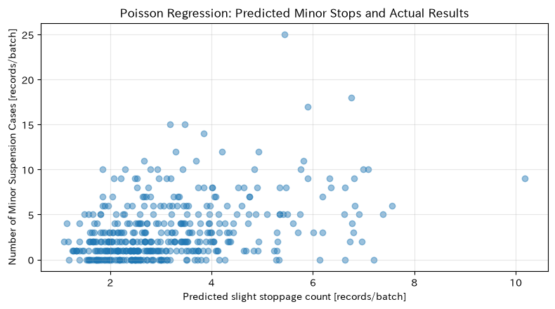
Pearson chi-square / Degrees of freedom: 2.832

Reading the results

exp(coefficient) is the rate of slight stops per unit increase. Using offset, the length of operating time is not estimated as an explanatory variable but is adjusted according to the exposure amount. On the other hand, if the Pearson chi square divided by degrees of freedom is well above 1, it is a sign of overdispersion, and Poisson’s standard error may be small. Along with the scattering of prediction points, consider the next negative binomial regression.

No.067: Negative Binomial Regression — Incorporating the Overdispersance of Microstops

Meaning in Practice

Minor stoppages are concentrated on days when unobserved factors such as material lots and equipment conditions overlap. Ignoring daily differences that cannot be expressed by average number of cases narrows the range for judging “abnormal” and can lead to excessive alerts.

Approach to Analysis and Modeling

Negative binary regression also uses logarithmic linking, but the variance

$$\mathrm{Var}(Y_i\mid X_i)=\mu_i+\alpha\mu_i^2$$

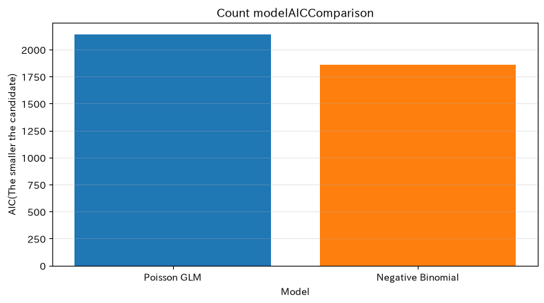
and allow overdistribution at $\alpha>0$. Poisson is the extreme of $\alpha\to0$. AIC is a comparative metric of fit and complexity between models applied to the same data, with the smaller option as a candidate.

Check with Python

nb_model = sm.NegativeBinomial(
    df["micro_stops"], X_count, offset=np.log(df["operating_hours"])
).fit(disp=False)
nb_params = nb_model.params
nb_table = pd.DataFrame({
    "estimated value": nb_params,
    "exp(estimated value)": np.exp(nb_params),
    "pvalue": nb_model.pvalues,
})
display(nb_table.round(4))
comparison_count = pd.DataFrame({
    "Model": ["Poisson GLM", "Negative Binomial"],
    "AIC": [poisson_model.aic, nb_model.aic],
    "Log likelihood": [poisson_model.llf, nb_model.llf],
})
display(comparison_count.round(2))

plt.bar(comparison_count["Model"], comparison_count["AIC"], color=["tab:blue", "tab:orange"])
plt.title("Count modelAICComparison")
plt.xlabel("Model")
plt.ylabel("AIC(The smaller the candidate)")
plt.grid(True, axis="y", alpha=0.3)
plt.tight_layout()
plt.show()

	estimated value	exp(estimated value)	pvalue
const	-1.9694	0.1395	0.0
vibration	0.4821	1.6195	0.0
maintenance_days	0.0083	1.0083	0.0
alpha	0.5726	1.7729	0.0

	Model	AIC	Log likelihood
0	Poisson GLM	2141.00	-1067.50
1	Negative Binomial	1858.13	-925.06

Reading the results

If alpha is positive and the AIC of the negative binomial regression is smaller than Poisson, it is valuable to express overdispersion including unobserved heterogeneity. The exp of the coefficient is the incidence ratio, but alpha is not the effect of the explanatory variable. If zeros are extremely high, time-dependent, or in-facility correlations, zero excess models, mixed models, and time series models are also candidates.

No.068: GLM — Expressing Distorted Recovery Man-Hours with Gamma Regression

Meaning in Practice

The recovery effort is greater than zero, and a small number of long hours of work can cause distortion to the right. Since linear regression with normal error can produce negative predictions, Gamma distributions and logarithmic links that fit positive continuous quantities are used.

Approach to Analysis and Modeling

The Generalized Linear Model (GLM) combines probability distributions with linkage functions. In Gamma Regression,

$$Y_i\sim\mathrm{Gamma},\qquad \log E(Y_i\mid X_i)=\beta_0+x_i^T\beta$$

and always keep the forecasted average positive. The coefficient converted to an exponential $e^{\beta_j}$ is the multiplier of the average work-hours, and $(e^{\beta_j}-1)\times100\%$ is generally the relative rate of change.

Check with Python

gamma_features = ["vibration", "maintenance_days"]
X_gamma = sm.add_constant(df[gamma_features])
gamma_model = sm.GLM(
    df["recovery_hours"], X_gamma,
    family=sm.families.Gamma(link=sm.families.links.Log()),
).fit()
gamma_table = pd.DataFrame({
    "coefficient": gamma_model.params,
    "Average Workload Multiplier": np.exp(gamma_model.params),
    "pvalue": gamma_model.pvalues,
})
display(gamma_table.round(4))

gamma_pred = gamma_model.predict(X_gamma)
plt.scatter(gamma_pred, df["recovery_hours"], alpha=0.45)
plt.title("Gamma GLM: Estimated recovery man-hours and actual results")
plt.xlabel("Predicted average recovery man-hours [hours]")
plt.ylabel("Actual Recovery Effort [hours]")
plt.grid(True, alpha=0.3)
plt.tight_layout()
plt.show()

	coefficient	Average Workload Multiplier	pvalue
const	-1.2942	0.2741	0.0
vibration	0.2387	1.2697	0.0
maintenance_days	0.0123	1.0124	0.0

Reading the results

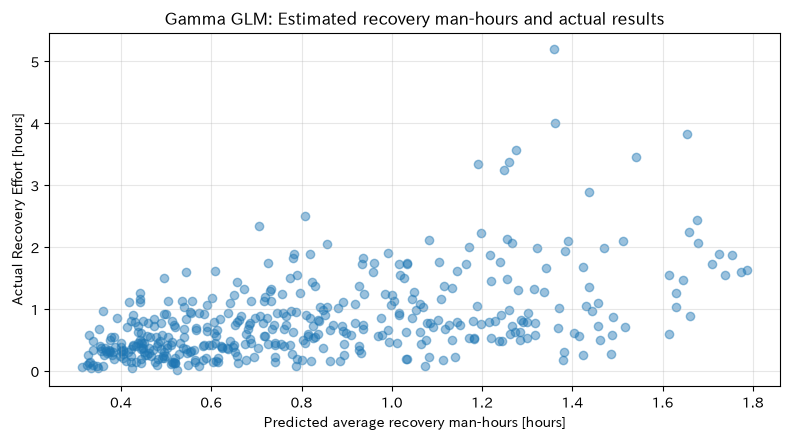
The predicted value of Gamma GLM remains positive, and the coefficient is interpreted as a multiplier rather than an addition time. For example, if you multiply the number of days after maintenance by 30, you can calculate the average workload multiplier for an increase of 30 days. Since changing the distribution does not mean the outlier is harmless, check residuals, impact points, and variety-specific fitting. GLM is an average model tailored to the distribution and does not accurately predict individual recovery times.

No.069: GAM — Capturing the Nonlinear Impact of Process Conditions

Meaning in Practice

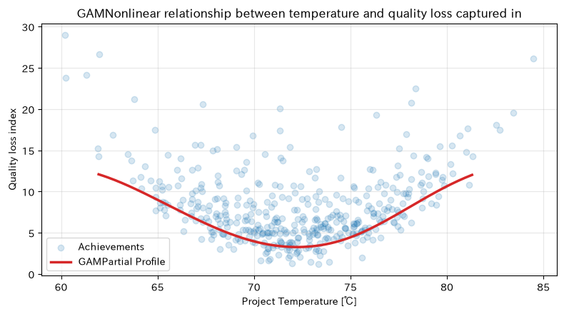
Quality loss is not always “worse when the temperature is higher”; it can worsen if the temperature is too low or too high. Since straight lines alone cannot represent a safe operating zone, it learns the effects of each variable using smooth curves.

Approach to Analysis and Modeling

The generalized additive model (GAM) is

$$g\{E(Y\mid X)\}=\beta_0+f_1(x_1)+f_2(x_2)+\cdots+f_p(x_p)$$

and $f_j$ is expressed as the weighted sum of the spline base. Here, each column is expanded to the B spline, and an additive model is created using Ridge to suppress excessive curve shaking. Because it does not include interactions, it is easy to explain, but it does not represent the combined effect of temperature × speed.

Check with Python

gam_features = ["temperature", "speed", "vibration"]
Xg_train, Xg_test, yg_train, yg_test = train_test_split(
    df[gam_features], df["quality_loss"], test_size=0.25, random_state=SEED
)
linear_quality = LinearRegression().fit(Xg_train, yg_train)
gam = make_pipeline(
    SplineTransformer(n_knots=6, degree=3, include_bias=False), Ridge(alpha=2.0)
).fit(Xg_train, yg_train)
print(f"linear model ReceptionRMSE: {mean_squared_error(yg_test, linear_quality.predict(Xg_test))**0.5:.3f}")
print(f"GAMequivalent   ReceptionRMSE: {mean_squared_error(yg_test, gam.predict(Xg_test))**0.5:.3f}")

temp_grid = np.linspace(df.temperature.quantile(0.01), df.temperature.quantile(0.99), 160)
profile = pd.DataFrame({
    "temperature": temp_grid,
    "speed": df.speed.median(),
    "vibration": df.vibration.median(),
})
plt.scatter(df.temperature, df.quality_loss, alpha=0.18, label="Achievements")
plt.plot(temp_grid, gam.predict(profile), color="tab:red", lw=2.5, label="GAMPartial Profile")
plt.title("GAMNonlinear relationship between temperature and quality loss captured in")
plt.xlabel("Project Temperature [℃]")
plt.ylabel("Quality loss index")
plt.grid(True, alpha=0.3)
plt.legend()
plt.tight_layout()
plt.show()

Linear Model Rating RMSE: 4.754
GAM Equivalent Rating RMSE: 1.769

Reading the results

Evaluation of GAM equivalent models compared to linear models If the RMSE is smaller and the partial profile is U-shaped, it suggests a favorable intermediate temperature range. However, the curve edges have little data and are unstable. The chart is a conditional forecast fixing speed and vibration at the median, not a simple scatter plot average. Before reflecting in the set standard, we examine validation experiments, interactions, and confidence intervals within acceptable limits.

No.070: Quantile Regression — Estimating the Upside Risk of Prolonged Batches

Meaning in Practice

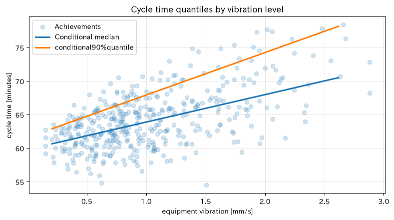
If you determine personnel and the capacity of subsequent processes solely by average cycle time, you overlook the conditions where delays tend to concentrate. Quile regression can directly model the median or 90% quantile and be used for planning at a level where “about one in ten exceeds this.”

Approach to Analysis and Modeling

$\tau$ Quintile regression is an asymmetric check loss

$$\rho_\tau(u)=u\{\tau-\mathbb{1}(u<0)\}$$

Minimize the total of the total. $\tau=0.5$ is the conditional median, and $\tau=0.9$ is the conditional 90th percentile. When the variance of error varies depending on conditions, changes in upside risk that cannot be seen in mean regression can be expressed as coefficients.

Check with Python

quant_features = ["speed", "vibration", "maintenance_days"]
X_quant = sm.add_constant(df[quant_features])
q50 = sm.QuantReg(df["cycle_time"], X_quant).fit(q=0.5)
q90 = sm.QuantReg(df["cycle_time"], X_quant).fit(q=0.9)
quant_table = pd.DataFrame({"median q=0.5": q50.params, "upper side q=0.9": q90.params})
display(quant_table.round(3))

vib_grid = np.linspace(df.vibration.quantile(0.01), df.vibration.quantile(0.99), 160)
quant_profile = pd.DataFrame({
    "const": 1.0, "speed": df.speed.median(), "vibration": vib_grid,
    "maintenance_days": df.maintenance_days.median(),
})
plt.scatter(df.vibration, df.cycle_time, alpha=0.2, label="Achievements")
plt.plot(vib_grid, q50.predict(quant_profile), lw=2.2, label="Conditional median")
plt.plot(vib_grid, q90.predict(quant_profile), lw=2.2, label="conditional90%quantile")
plt.title("Cycle time quantiles by vibration level")
plt.xlabel("equipment vibration [mm/s]")
plt.ylabel("cycle time [minutes] ")
plt.grid(True, alpha=0.3)
plt.legend()
plt.tight_layout()
plt.show()

	median q=0.5	upper side q=0.9
const	41.485	47.253
speed	0.149	0.113
vibration	4.090	6.336
maintenance_days	0.015	0.019

Reading the results

The lines at the 90th percentile represent the lower end of about 90% of the cycle time under each condition. If the vibration coefficient is greater than the median at the 90th percentile, it suggests that the oscillation is not only typical but also extends the long-term tail. For delivery dates and workforce planning, the upper quantile is used, while the representative standard work value is the median, selecting quantiles according to losses. Note that this differs from the simultaneous forecast interval for future values.

Practical Implications Seen Through Target Exercise

1. Select models based on the scale of the objective variable: For continuous quantities, binomies, number of cases, and positive distorted quantities, the reasonable distribution and links differ.
2. Adding the perspective of stability to correlation variables: Strategies are not decided solely by OLS coefficients; instead, predictions, conciseness, and reproducibility are compared using Ridge, Lasso, and ElasticNet.
3. Do not ignore exposure and overdispersion: The number of stoppages is adjusted by operating hours, and if variation exceeds the average, negative binomial regression is considered.
4. Only the averageKPInot to: By capturing nonlinear safety areas with GAM and upside risk with quantile regression, you can design condition standards and capability planning separately.
5. Distinguishing between prediction and causality: Even high-precision models do not guarantee the effectiveness of manipulating conditions. Implementing improvements requires on-site knowledge and verification experiments.

What is necessary for practical implementation

1. Define the timing of prediction and decision-making

First, decide when, who, and what predictions to change. If you include information that becomes known after the prediction point into the explanatory variable, it results in a data leak with high verification accuracy.

2. Manage the data generation process

Unit, missing items, sensor calibration, equipment/type/worker ID, operating hours, and maintenance history are all provided. Random segmentation that ignores repeated observations of the same equipment or time-series segmentation can sometimes make performance appear optimistic.

3. Evaluate model selection and thresholds based on operational losses

We translate not only RMSE, AUC, and AIC, but also missed non-conformity costs, additional inspection costs, downtime alert response costs, and personnel shortage losses. Learning, validation, and final evaluation are separated, and hyperparameters are determined through validation data or cross-validation.

4. Determine post-operation monitoring and responsibility separation

Continuously monitor input distribution, loss rate, calibration, residuals, and performance-specific equipment levels. It clearly states the scope of decision support the model, conditions that the field can overturn, criteria for relearning and stopping, and change history.

5. Verify the effect of improvement through experiments

Based on the regression coefficients, we create improvement hypotheses and implement DOE or phased implementations within safe and quality limits. We will separate the relationship between the predictive model and the causal effects resulting from configuration changes.

Conclusion

From No.061 to No.070, it was confirmed that even with the same manufacturing data, the need to change models according to the target variable and decision was confirmed.

• Correlation and variable count were controlled using linear regression as the baseline, using Ridge, Lasso, and ElasticNet
• Modeled the probability of nonconformance using logistic regression and the slight stops per uptime using Poisson/negative binary regression
• Gamma GLM identified positive distorted man-hours, GAM used nonlinear relationships, and quantile regression captured upside risk.

In practice, what’s important is not choosing the most complex model. It is about clarifying the mechanism of data generation and its intended use, verifying it with unknown data, and connecting forecasts to decisions on cost, quality, and delivery schedules.

Consultations for Corporations

At Suri Kobo, we can provide the following support for the manufacturing industry.

• Design and validation of predictive models using quality, equipment, and production performance
• Selection of GLM and machine learning based on nonconformities, number of outages, and recovery effort
• Designing KPIs, thresholds, and monitoring methods from PoC to field operations
• Corporate training on regression analysis, statistical modeling, and Python utilization

Even at the stage where “I want to organize what can be predicted with my current data” or “I’ve achieved accuracy but it doesn’t lead to on-site decision-making,” I proceed while checking business challenges and the data generation process.

📩 Contact Us: surikobo.co.jp/contact
Please feel free to consult us first.