Don’t End Improvement Effects as ‘Accidents’: 10 Exercise-Ups in Hypothesis Testing in Manufacturing

On the manufacturing floor, various comparisons are made daily, such as changing equipment conditions, updating jigs, switching suppliers, and checking after maintenance. However, simply seeing differences in sample mean or number of nonconformities does not distinguish whether the difference is due to process changes or coincidental variation.

In this article, we will implement tFrom the certification examLjung–BoxUp to the Certification10Types of Hypothesis Testing using Python as the subject of a fictional precision parts factory. Rather than memorizing test names, we focus on checking data correspondences, distributions, sample sizes, variances, and time series dependence, and connecting them to decision-making along with effect sizes and confidence intervals.

[!NOTE] This material is a notebook previously used by Surikoubo (or personally by the representative, Kazuyama), and has been reconstructed, edited, and published with the company’s permission.
All data listed is fictional and has no relation whatsoever to real companies, factories, or figures.

Introduction: Practical Challenges in Manufacturing Covered in This Article

The theme this time is “Turning observed differences into grounds for adopting changes.” We address questions such as whether the filling amount deviates from standards, whether power consumption has decreased due to energy-saving settings, whether there are dimensional differences between lines, and whether strength varies depending on the supplier.

Hypothesis testing calculates the p-value, which is the probability that data will be more extreme than the observation results under null hypothesis $H_0$. A small p-value indicates “low consistency between $H_0$ and data,” but it does not directly indicate the magnitude of the improvement or the value of the investment. In this article, while the significance level is generally set as $alpha=0.05$, we also list the differences, effect sizes, confidence intervals, and assumptions.

Common situations on site

• Comparing only the average before and after improvement concludes, ‘It decreased, so it works.’
• Treat data measured before and after changing the same equipment as two independent groups
• For line comparisons with significantly different variances, a test assuming equal variance is used
• Use tests with unstable approximations for nonconformities with few occurrences
• Mechanical use of mean-based tests for data containing non-normal and outlier values
• Treat time-series data as independent samples and overlook continuous biases

Mischoosing the testing method leads to horizontal rollout of ineffective changes, delaying necessary improvements, and underestimating quality risks.

Why is this issue so difficult to judge?

Statistical differences and practical differences are not the same. If the sample size is large, even very small differences can be significant, while if the sample size is small, it may not be possible to detect significant differences. Also, repeating multiple tests increases the probability of finding chance and significant differences.

In practice, the following points must be defined before the exam.

1. Comparative unit: Product, lot, equipment, day, or worker
2. Relationship: Whether the same object was compared before and after or as an independent group.
3. Key Evaluation Indicators: Mean or median, ratio, distribution shape, or autocorrelation
4. Least Importance Deviation: Some meaningful differences from a field perspective
5. Analysis Plan: One-sided and two-sided, significance levels, exclusion rules, handling multiple comparisons

Testing becomes a repeatable decision only with this design.

Overview of Exercise covered this time

No.	technique	Fictitious Practical Challenges	Main Things to Check
051	t-test	Is the average filling amount different from the standard value?	Group Mean
052	Supported t-Test	Did the power supply change before or after changing the settings of the same equipment?	Mean of correspondence differences
053	Welch Certification	Do the two lines with different variation have different dimensional averages?	Mean of two independent groups
054	chi-square test	Is there a connection between shift and nonconformity classification?	Independence Between Categories
055	Fisher Exact Testing	Are there a few incidents related to firmware and outage alarms?	2×2 Table Ratio
056	ANOVA	3. Is the average breaking load of suppliers different?	Mean of three or more independent groups
057	Mann–Whitney Test	2. Is there a difference in the setting time for non-standard jigs?	Standings of Independent Group 2
058	Kruskal–Wallis Test	3. Is the distribution of recovery times for the conservation teams different?	Standings of Independent Groups 3 or More
059	Kolmogorov–Smirnov Test	Does the cycle time match the pre-reference distribution?	overall distribution
060	Ljung–Box Certification	Check if there is any time series dependence left in the furnace temperature model residual.	Multi-lug autocorrelation

Preparing the Python environment

Generate fictitious data with NumPy, organize tables with pandas, and perform tests with SciPy. Graphs use matplotlib, and Japanese display uses japanize-matplotlib. The random number generator is created only once, and by fixing the seed, the same result is reproduced each time it runs.

import platform

import matplotlib
import matplotlib.pyplot as plt
import japanize_matplotlib
import numpy as np
import pandas as pd
import scipy
from IPython.display import display
from scipy import stats

SEED = 202606
rng = np.random.default_rng(SEED)
ALPHA = 0.05

pd.set_option("display.precision", 4)
plt.rcParams["figure.figsize"] = (8, 4.5)
plt.rcParams["axes.unicode_minus"] = False

print(f"Python     : {platform.python_version()}")
print(f"NumPy      : {np.__version__}")
print(f"pandas     : {pd.__version__}")
print(f"SciPy      : {scipy.__version__}")
print(f"matplotlib : {matplotlib.__version__}")
print(f"random numberseed   : {SEED}")

Python     : 3.13.1
NumPy      : 2.5.1
pandas     : 3.0.3
SciPy      : 1.18.0
matplotlib : 3.11.0
Random seed: 202606

Creation of Fictional Data

We assume process capability checks, equipment improvements, quality classification, supplier evaluations, and maintenance evaluations conducted within a single factory. No external files are used; continuous quantities are created from normal distribution or long distribution at the right end, category data is aggregated tables, and time series residuals are created from autoregressive processes.

While differences are embedded during data generation, in practice, it is not possible to recollect data until the expected results are achieved. It is important to determine sample size, key indicators, and exclusion criteria before analysis.

# No.051: Filling Amount (g), Standard 500 g
fill_weight = rng.normal(loc=500.48, scale=1.10, size=40)

# No.052: Power consumption per batch of 12 units of the same equipment (kWh)
energy_before = rng.normal(loc=126.0, scale=5.0, size=12)
energy_after = energy_before - rng.normal(loc=4.2, scale=2.0, size=12)

# No.053: Shaft diameter deviation (μm) of line A/B. B has a small sample size and large variance
diameter_a = rng.normal(loc=0.00, scale=0.16, size=36)
diameter_b = rng.normal(loc=0.16, scale=0.38, size=22)

# No.054: Row=Shift, Column=Nonconformity Classification
defect_table = pd.DataFrame(
    [[18, 7, 5], [8, 17, 15]],
    index=["day shift", "night shift"], columns=["Exterior", "Dimensions", "foreign object"]
)

# No.055: Row = old/new firmware, Column = With or without stop alarm
alarm_table = pd.DataFrame(
    [[7, 23], [1, 29]],
    index=["Old edition", "New Edition"], columns=["Stop warning", "No stop alarm"]
)

# No.056: Breaking Load (kN) of Three Suppliers
strength = {
    "supplierA": rng.normal(50.00, 0.18, 20),
    "supplierB": rng.normal(50.10, 0.18, 20),
    "supplierC": rng.normal(50.32, 0.18, 20),
}

# No.057: Setup time for two independent jigs (minutes, right hem is longer)
setup_old = rng.lognormal(mean=np.log(18.0), sigma=0.28, size=28)
setup_new = rng.lognormal(mean=np.log(15.5), sigma=0.25, size=26)

# No.058: Recovery time for three maintenance teams (may include minutes and outliers)
recovery = {
    "classA": rng.lognormal(np.log(38), 0.30, 18),
    "classB": rng.lognormal(np.log(31), 0.28, 18),
    "classC": rng.lognormal(np.log(47), 0.35, 18),
}

# No.059: Cycle time (seconds). Compared with a pre-fixed reference distribution N(45, 2.5^2)
cycle_time = 40.5 + rng.gamma(shape=2.0, scale=2.25, size=80)

# No.060: Residual (°C) of furnace temperature prediction model. Maintaining continuity as AR(1)
innovations = rng.normal(0, 0.55, 120)
temp_residual = np.zeros(120)
for t in range(1, len(temp_residual)):
    temp_residual[t] = 0.62 * temp_residual[t - 1] + innovations[t]

data_overview = pd.DataFrame({
    "Analysis Theme": ["Filling volume", "installed power", "shaft diameter deviation", "Unsuitable for classification", "stop alarm",
                 "breaking load", "Interval time", "Recovery Time", "cycle time", "Furnace Temperature Model Residual"],
    "Observation Unit/group": [len(fill_weight), len(energy_before), f"{len(diameter_a)} / {len(diameter_b)}",
                int(defect_table.to_numpy().sum()), int(alarm_table.to_numpy().sum()),
                " / ".join(str(len(v)) for v in strength.values()),
                f"{len(setup_old)} / {len(setup_new)}",
                " / ".join(str(len(v)) for v in recovery.values()), len(cycle_time), len(temp_residual)],
    "Certifications used": ["1speciment", "Responset", "Welch", "chi-square", "Fisher",
                "ANOVA", "Mann–Whitney", "Kruskal–Wallis", "KS", "Ljung–Box"],
})
display(data_overview)

	Analysis Theme	Observation Unit/group	Certifications used
0	Filling volume	40	1speciment
1	installed power	12	Responset
2	shaft diameter deviation	36 / 22	Welch
3	Unsuitable for classification	70	chi-square
4	stop alarm	60	Fisher
5	breaking load	20 / 20 / 20	ANOVA
6	Interval time	28 / 26	Mann–Whitney
7	Recovery Time	18 / 18 / 18	Kruskal–Wallis
8	cycle time	80	KS
9	Furnace Temperature Model Residual	120	Ljung–Box

No.051: t-test — Does the average filling amount differ from the reference value?

Meaning in Practice

Check whether the average filling process is off from the displayed 500 g mark. Overfilling leads to material loss, while underfilling leads to violations of customer requirements, so this is related to process-focused adjustment decisions. However, to guarantee compliance with standards, a separate process capability analysis is also required.

Approach to Analysis and Modeling

Let the null hypothesis $H_0:\mu=500$ and the alternative hypothesis $H_1:\mu\neq500$. The one-sample t-statistic with unknown population variance is

$$t=\frac{\bar{x}-\mu_0}{s/\sqrt{n}}$$

That’s right. Assuming the independence of observations and the ability to approximate the sample distribution of the mean, we assume t. In addition to p-values, the mean deviation, 95% confidence interval, and standardized effect size Cohen’s $d$ are checked.

Check with Python

target_weight = 500.0
t51 = stats.ttest_1samp(fill_weight, popmean=target_weight)
mean51 = fill_weight.mean()
sd51 = fill_weight.std(ddof=1)
ci51 = stats.t.interval(0.95, len(fill_weight) - 1, loc=mean51, scale=stats.sem(fill_weight))
d51 = (mean51 - target_weight) / sd51

display(pd.DataFrame({
    "average[g]": [mean51], "Difference from the standard[g]": [mean51 - target_weight],
    "95%CIlower_limit": [ci51[0]], "95%CIupper": [ci51[1]],
    "tvalue": [t51.statistic], "pvalue": [t51.pvalue], "Cohen's d": [d51],
    "determination(alpha=0.05)": ["Differences from standards" if t51.pvalue < ALPHA else "Unable to confirm the difference,"]
}))

fig, ax = plt.subplots()
ax.hist(fill_weight, bins=10, color="#4C78A8", edgecolor="white", alpha=0.85)
ax.axvline(target_weight, color="#E45756", linestyle="--", label="standard 500 g")
ax.axvline(mean51, color="#2A9D8F", linewidth=2, label=f"specimen mean {mean51:.2f} g")
ax.set_title("Distribution and reference values of filling volume")
ax.set_xlabel("Filling volume [g]")
ax.set_ylabel("quantity")
ax.grid(axis="y", alpha=0.3)
ax.legend()
plt.tight_layout()
plt.show()

	average[g]	Difference from the standard[g]	95%CIlower_limit	95%CIupper	tvalue	pvalue	Cohen's d	determination(alpha=0.05)
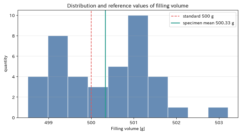
0	500.3297	0.3297	499.9755	500.6839	1.8827	0.0672	0.2977	Unable to confirm the difference,

Reading the results

The output averages over 500 g, and deviations in process centers can be evaluated from the 95% confidence interval and p-value. However, even if there is a statistical difference, if the difference is small compared to adjustment costs or the uncertainty of the meter, immediate adjustment may not be the best option. Determine the minimum importance difference in advance and adjust after checking the stability in the time direction on the control chart.

No.052: Compatible t-Certification — Comparing Before and After Energy-Saving Settings for the Same Equipment

Meaning in Practice

For the same 12 units, compare the power consumption per batch before and after the setting change. By subtracting the fundamental differences in consumption between equipment, it becomes easier to evaluate the effectiveness of the setting changes themselves.

Approach to Analysis and Modeling

If the difference in equipment $i$ is $d_i=x_{\mathrm{before},i}-x_{\mathrm{after},i}$, the corresponding t-test is a one-sample t-test that tests $H_0:\mu_d=0$. The important assumption is not the normality of the front and back, but poor $d_i$ Independence and Approximate Normality. Do not compromise the compatibility of the same equipment.

Check with Python

diff52 = energy_before - energy_after
t52 = stats.ttest_rel(energy_before, energy_after)
ci52 = stats.t.interval(0.95, len(diff52) - 1, loc=diff52.mean(), scale=stats.sem(diff52))

display(pd.DataFrame({
    "Average before change[kWh]": [energy_before.mean()], "Average after change[kWh]": [energy_after.mean()],
    "Average reduction[kWh]": [diff52.mean()], "Amount reduced95%CIlower_limit": [ci52[0]],
    "Amount reduced95%CIupper": [ci52[1]], "tvalue": [t52.statistic], "pvalue": [t52.pvalue],
    "determination": ["There is a difference between front and rear" if t52.pvalue < ALPHA else "Unable to check the difference before and after,"]
}))

fig, ax = plt.subplots()
for i, (before, after) in enumerate(zip(energy_before, energy_after), start=1):
    ax.plot(["Before the change", "After the change"], [before, after], marker="o", alpha=0.55)
ax.set_title("Power consumption before and after changing the same equipment settings")
ax.set_xlabel("Setting")
ax.set_ylabel("1Power consumption per batch [kWh]")
ax.grid(alpha=0.3)
plt.tight_layout()
plt.show()

	Average before change[kWh]	Average after change[kWh]	Average reduction[kWh]	Amount reduced95%CIlower_limit	Amount reduced95%CIupper	tvalue	pvalue	determination
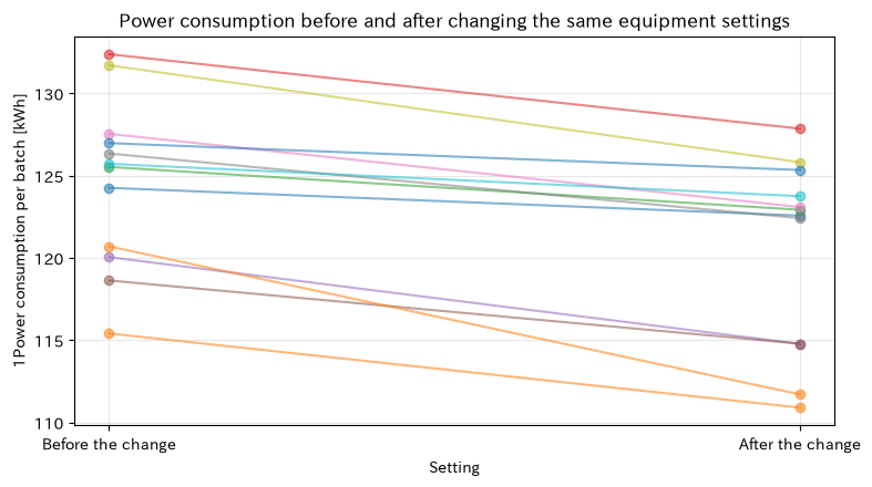
0	124.6055	120.4945	4.1109	2.7853	5.4366	6.8255	2.8555e-05	There is a difference between front and rear

Reading the results

If many lines are trending downward to the right and the confidence interval for average savings does not cross zero, it is a factor supporting energy-saving effects. Before horizontal rollout, we check the conditions that have changed before and after such as production volume, variety, outside temperature, and startup time. When converted into annual batch numbers and electricity unit prices, the amount of electricity saved can be explained as practical investment effects.

No.053: Welch Test — Comparing the Dimensional Averages of Two Lines with Different Variation

Meaning in Practice

Compare the axis diameter deviations of lines A and B. B is expected to have a small sample size and significant variation depending on equipment condition and material lot size. Before performing inter-line correction, evaluate whether the mean deviation is within the coincidental range.

Approach to Analysis and Modeling

Welch’s t-test tests the mean difference between two independent groups without assuming equal variance. The statistics are

$$t=\frac{\bar{x}_A-\bar{x}_B}{\sqrt{s_A^2/n_A+s_B^2/n_B}}$$

The degrees of freedom are determined using the Welch–Satterthwaite approximation. If there is a strong series correlation in products taken continuously from equipment, independent analytical units are designed, such as consolidating them to the lot level.

Check with Python

t53 = stats.ttest_ind(diameter_a, diameter_b, equal_var=False)
va, vb = diameter_a.var(ddof=1), diameter_b.var(ddof=1)
se53 = np.sqrt(va / len(diameter_a) + vb / len(diameter_b))
df53 = (va / len(diameter_a) + vb / len(diameter_b)) ** 2 / (
    (va / len(diameter_a)) ** 2 / (len(diameter_a) - 1)
    + (vb / len(diameter_b)) ** 2 / (len(diameter_b) - 1)
)
diff53 = diameter_a.mean() - diameter_b.mean()
ci53 = diff53 + np.array([-1, 1]) * stats.t.ppf(0.975, df53) * se53

display(pd.DataFrame({
    "Aaverage[μm]": [diameter_a.mean()], "Baverage[μm]": [diameter_b.mean()],
    "Astandard_deviation": [np.sqrt(va)], "Bstandard_deviation": [np.sqrt(vb)],
    "mean deviationA-B": [diff53], "difference95%CIlower_limit": [ci53[0]], "difference95%CIupper": [ci53[1]],
    "Welchdegree of freedom": [df53], "tvalue": [t53.statistic], "pvalue": [t53.pvalue],
}))

fig, ax = plt.subplots()
ax.boxplot([diameter_a, diameter_b], tick_labels=["LineA", "LineB"], showmeans=True)
ax.axhline(0, color="#E45756", linestyle="--", label="Design Center")
ax.set_title("Shaft diameter deviation by line")
ax.set_xlabel("Production Line")
ax.set_ylabel("shaft diameter deviation [μm]")
ax.grid(axis="y", alpha=0.3)
ax.legend()
plt.tight_layout()
plt.show()

	Aaverage[μm]	Baverage[μm]	Astandard_deviation	Bstandard_deviation	mean deviationA-B	difference95%CIlower_limit	difference95%CIupper	Welchdegree of freedom	tvalue	pvalue
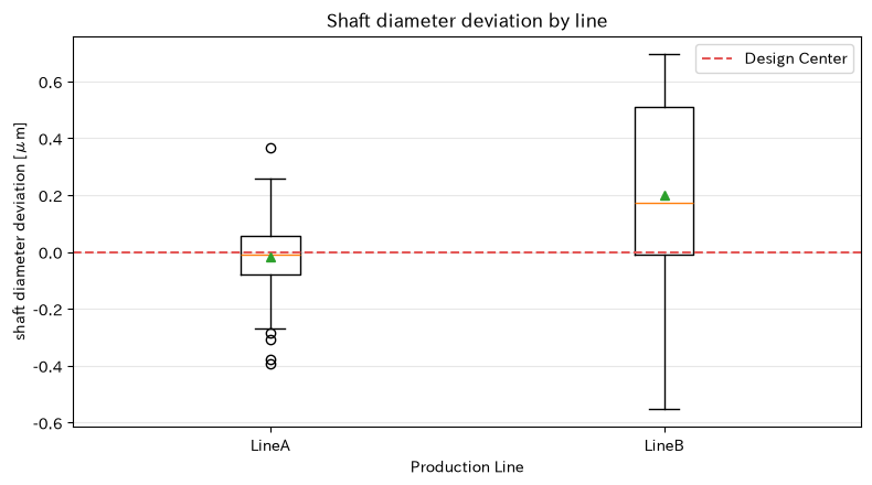
0	-0.0185	0.1991	0.1734	0.3552	-0.2176	-0.3839	-0.0513	27.2124	-2.6841	0.0122

Reading the results

The Welch test evaluates the mean difference by incorporating differences in sample size and variance. From the box beard chart, you can see not only the average difference but also the large variation in B. Since averaging alone may not be sufficient to eliminate quality risks, B prioritizes confirming the layers of variation factors and process capability.

No.054: Chi-square Test — Investigating the Relationship Between Shift and Nonconformity Classification

Meaning in Practice

We check whether the non-conformity configurations of appearance, dimensions, and foreign objects are the same between day and night shifts. Identify differences in composition ratios that cannot be seen from the total number of nonconformities alone, and determine priorities such as lighting, planning, cleaning, and inspection education.

Approach to Analysis and Modeling

In the chi-square test of independence, the null hypothesis is defined as “the shift and nonconformity classification are independent.” The expected level is

$$E_{ij}=\frac{(i\text{total of rows})(j\text{total of columns})}{\text{total number}},\qquad \chi^2=\sum_{i,j}\frac{(O_{ij}-E_{ij})^2}{E_{ij}}$$

That’s right. If there are many cells with low expected degrees, the approximation becomes unstable. Look at the standardized residual $(O-E)/\sqrt{E}$ to see which combinations contributed to the difference.

Check with Python

chi54, p54, dof54, expected54 = stats.chi2_contingency(defect_table)
expected54 = pd.DataFrame(expected54, index=defect_table.index, columns=defect_table.columns)
residual54 = (defect_table - expected54) / np.sqrt(expected54)

display(pd.concat({"Observation frequency": defect_table, "Expected Degree": expected54.round(2),
                   "Pearsonresidual": residual54.round(2)}, axis=1))
display(pd.DataFrame({"Chi-square value": [chi54], "degree of freedom": [dof54], "pvalue": [p54],
                      "Minimum expected degree": [expected54.min().min()],
                      "determination": ["Related" if p54 < ALPHA else "Unable to confirm the connection"]}))

rates54 = defect_table.div(defect_table.sum(axis=1), axis=0)
ax = rates54.plot(kind="bar", color=["#4C78A8", "#F2CF5B", "#E45756"])
ax.set_title("Composition ratio of nonconformity classifications by shift")
ax.set_xlabel("Work Shift")
ax.set_ylabel("Shift Composition Ratio")
ax.grid(axis="y", alpha=0.3)
ax.legend(title="Unsuitable for classification")
plt.xticks(rotation=0)
plt.tight_layout()
plt.show()

	Observation frequency			Expected Degree			Pearsonresidual
	Exterior	Dimensions	foreign object	Exterior	Dimensions	foreign object	Exterior	Dimensions	foreign object
day shift	18	7	5	11.14	10.29	8.57	2.05	-1.02	-1.22
night shift	8	17	15	14.86	13.71	11.43	-1.78	0.89	1.06

	Chi-square value	degree of freedom	pvalue	Minimum expected degree	determination
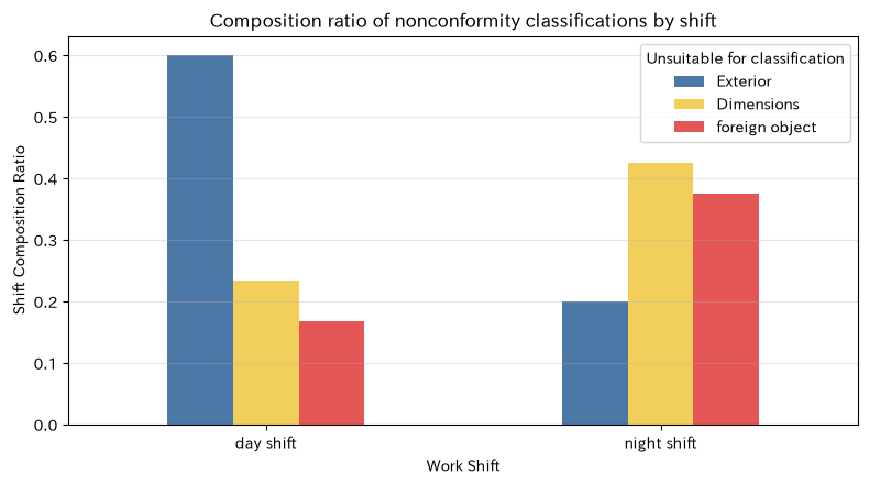
0	11.8256	2	0.0027	8.5714	Related

Reading the results

If the p-value is small, it is difficult to consider the shift and nonconformity classification as independent. From the composition ratio and residuals, you can see that the structure has more dimensions and foreign objects during the day shift, while the day shift has more dimensions and foreign objects. However, the shift itself is not always the cause; we track whether product composition, material lots, equipment, and inspectors are all mixed up.

No.055: Fisher Exact Test — Evaluating a Small Number of Stop Alarms Using a 2×2 Table

Meaning in Practice

Testing both old and new firmware for sensor control on 30 devices is conducted to aggregate the presence or absence of a stop alarm. Even when the number of incidents is low, it’s important to evaluate whether the new version is related to the alert rate.

Approach to Analysis and Modeling

The Fisher exact test calculates the probability of tables more extreme than observation tables from conditional distributions with fixed marginal frequencies in 2×2 partition tables. It is useful when the sample size is small or the expected degree is small. odds ratio

$$\mathrm{OR}=\frac{ad}{bc}$$

Also mentioned here. Here, since it’s ‘Old Version Warning Odds / New Version Warning Odds,’ the higher the number of warnings from the old version, the higher the number of warnings above 1.

Check with Python

odds55, p55 = stats.fisher_exact(alarm_table.to_numpy(), alternative="two-sided")
rates55 = alarm_table["Stop warning"] / alarm_table.sum(axis=1)

display(alarm_table)
display(pd.DataFrame({
    "Older Alert Rate": [rates55["Old edition"]], "New Alert Rate": [rates55["New Edition"]],
    "Alarm rate difference(old-new)": [rates55["Old edition"] - rates55["New Edition"]],
    "odds ratio(old/new)": [odds55], "both sidespvalue": [p55],
    "determination": ["Related" if p55 < ALPHA else "Unable to confirm the connection"]
}))

fig, ax = plt.subplots()
ax.bar(rates55.index, rates55.values, color=["#E45756", "#2A9D8F"])
ax.set_title("Stop Alarm Rate by Firmware")
ax.set_xlabel("firmware")
ax.set_ylabel("Stop alarm rate")
ax.set_ylim(0, max(rates55.max() * 1.3, 0.1))
ax.grid(axis="y", alpha=0.3)
plt.tight_layout()
plt.show()

	Stop warning	No stop alarm
Old edition	7	23
New Edition	1	29

	Older Alert Rate	New Alert Rate	Alarm rate difference(old-new)	odds ratio(old/new)	both sidespvalue	determination
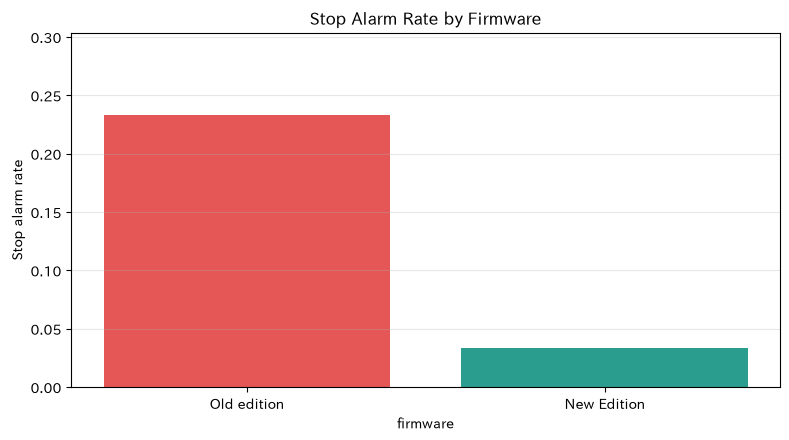
0	0.2333	0.0333	0.2	8.8261	0.0523	Unable to confirm the connection

Reading the results

The new version has a low alert rate, and the odds ratio also indicates the direction of effect. On the other hand, because the number of cases is small, p-values can become boundary. We cannot conclude that “not significant = equivalent.” For safety-related indicators, phased implementation is determined by considering the effectiveness direction, allowable risk, number of additional tests required, and the nature of serious events.

No.056: ANOVA — Comparing the average breaking loads of three suppliers

Meaning in Practice

We compare whether there is a difference in average fracture load among three companies supplying components with the same specifications. This is related to supplier certification and reviewing the level of acceptance inspection.

Approach to Analysis and Modeling

Univariate ANOVA uses $H_0:\mu_A=\mu_B=\mu_C$ as the ratio of between-group variation to intra-group variation

$$F=\frac{MS_{\mathrm{between}}}{MS_{\mathrm{within}}}$$

I will take the certification exam. Independence, approximate normality of each group, and uniform variance are prerequisites. Even if ANOVA is significant, it does not necessarily mean that “all combinations differ,” so prior or multiple comparisons are necessary. Here, we also check the overall effect size $\eta^2=SS_{\mathrm{between}}/SS_{\mathrm{total}}$ and Tukey HSD.

Check with Python

f56 = stats.f_oneway(*strength.values())
all56 = np.concatenate(list(strength.values()))
grand56 = all56.mean()
ss_between56 = sum(len(x) * (x.mean() - grand56) ** 2 for x in strength.values())
ss_total56 = ((all56 - grand56) ** 2).sum()
eta56 = ss_between56 / ss_total56
tukey56 = stats.tukey_hsd(*strength.values())

display(pd.DataFrame({
    "n": [len(x) for x in strength.values()],
    "average[kN]": [x.mean() for x in strength.values()],
    "standard_deviation[kN]": [x.std(ddof=1) for x in strength.values()],
}, index=strength.keys()))
display(pd.DataFrame({"Fvalue": [f56.statistic], "pvalue": [f56.pvalue], "etasquare": [eta56],
                      "determination": ["at least1There are differences among the flocks." if f56.pvalue < ALPHA else "Unable to confirm the difference,"]}))
display(pd.DataFrame(tukey56.pvalue, index=strength.keys(), columns=strength.keys()).round(4))

fig, ax = plt.subplots()
ax.boxplot(list(strength.values()), tick_labels=list(strength.keys()), showmeans=True)
ax.set_title("Breaking Load by Supplier")
ax.set_xlabel("supplier")
ax.set_ylabel("breaking load [kN]")
ax.grid(axis="y", alpha=0.3)
plt.tight_layout()
plt.show()

	n	average[kN]	standard_deviation[kN]
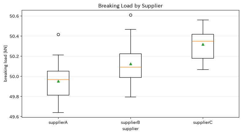
supplierA	20	49.9516	0.1885
supplierB	20	50.1246	0.2153
supplierC	20	50.3190	0.1516

	Fvalue	pvalue	etasquare	determination
0	19.3208	3.9264e-07	0.404	at least1There are differences among the flocks.

	supplierA	supplierB	supplierC
supplierA	1.0000	0.0135	0.0000
supplierB	0.0135	1.0000	0.0049
supplierC	0.0000	0.0049	1.0000

Reading the results

The p-value of ANOVA indicates whether there is an overall average variation, while $\eta^2$ indicates how much the supplier explains the total variation. You can narrow down combinations with differences using Tukey HSD’s p-value matrix. However, suppliers with higher average standards are not always optimal. We design certification standards that include margins, variation, price, delivery time, and changes between lots relative to the minimum standard limit.

No.057: Mann–Whitney Test — Comparing the Setup Time of Two Jigs by Ranking

Meaning in Practice

Use the old jig and the new jig for separate tasks, and evaluate whether there is a difference in the distribution of setup times. Since the setup time does not fall below zero and the right hem tends to be long during troubles, it is a difficult indicator to handle assuming average values and normal distributions.

Approach to Analysis and Modeling

The Mann–Whitney U test is a nonparametric test that ranks two independent groups together and evaluates ranking bias. If the distribution shapes of the two groups are considered the same, it can be interpreted as a difference in position, but if the shapes are also different, it cannot be called a “median-only test.” Here, the median, quartile range, and ranking binary correlation are also listed.

Check with Python

u57 = stats.mannwhitneyu(setup_old, setup_new, alternative="two-sided")
rbc57 = 2 * u57.statistic / (len(setup_old) * len(setup_new)) - 1

summary57 = pd.DataFrame({
    "n": [len(setup_old), len(setup_new)],
    "median[minutes]": [np.median(setup_old), np.median(setup_new)],
    "No.1quartile": [np.quantile(setup_old, .25), np.quantile(setup_new, .25)],
    "No.3quartile": [np.quantile(setup_old, .75), np.quantile(setup_new, .75)],
}, index=["Old fixture", "New fixture"])
display(summary57)
display(pd.DataFrame({"Uvalue": [u57.statistic], "pvalue": [u57.pvalue],
                      "Ranking binary correlation": [rbc57],
                      "determination": ["Differences in distribution locations" if u57.pvalue < ALPHA else "Unable to confirm the difference,"]}))

fig, ax = plt.subplots()
for values, label, color in [(setup_old, "Old fixture", "#E45756"), (setup_new, "New fixture", "#2A9D8F")]:
    x = np.sort(values)
    y = np.arange(1, len(x) + 1) / len(x)
    ax.step(x, y, where="post", label=label, color=color)
ax.set_title("Cumulative Distribution of Experience in Setup Time by Jig")
ax.set_xlabel("Interval time [minutes]")
ax.set_ylabel("Cumulative Percentage")
ax.grid(alpha=0.3)
ax.legend()
plt.tight_layout()
plt.show()

	n	median[minutes]	No.1quartile	No.3quartile
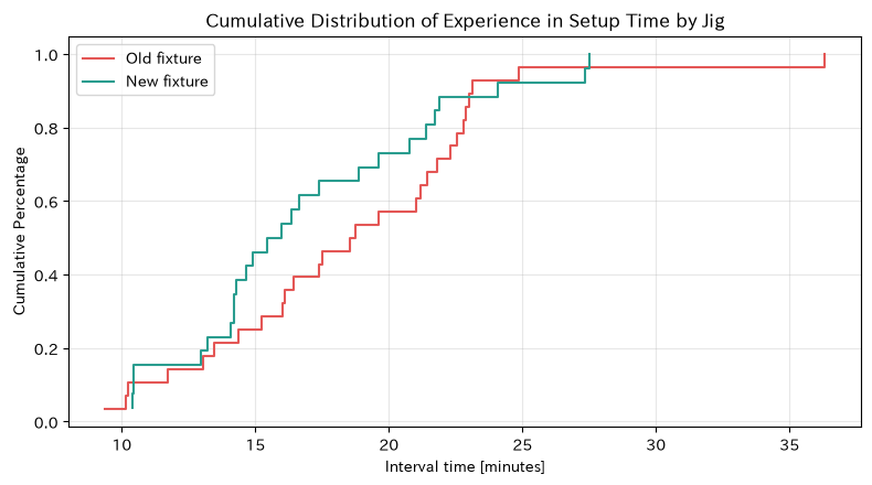
Old fixture	28	18.6360	15.0231	22.3628
New fixture	26	15.6962	14.1175	20.4698

	Uvalue	pvalue	Ranking binary correlation	determination
0	437.0	0.2094	0.2005	Unable to confirm the difference,

Reading the results

The more accumulated experience distribution is on the left, the faster the setup tends to be completed. In addition to p-values, the median difference and ranking binary correlation are used to check the magnitude of the difference. Since this is a comparison of independent groups, if the worker’s skill level or the difficulty of the variety is uneven, it can be mixed with the jig effect. If possible, design a random usage order using the same workers and similar product types.

No.058: Kruskal–Wallis Test — Ranking the recovery times of three maintenance teams

Meaning in Practice

Compare recovery times for the three maintenance teams and consider standardization of procedures and focus on education. Recovery times tend to be deviated depending on the difficulty of the failure, raising doubts about normality and equal distribution.

Approach to Analysis and Modeling

The Kruskal–Wallis test ranks three or more independent groups together and evaluates differences in average rankings among groups. The null hypothesis means that the distribution of each group is the same. Test statistic $H$ approximates a chi-square distribution with degrees of freedom $k-1$ in large samples. Even if the overall certification is significant, multiple comparisons are required separately to determine which groups are different.

Check with Python

h58 = stats.kruskal(*recovery.values())
n58 = sum(len(x) for x in recovery.values())
k58 = len(recovery)
epsilon58 = max(0, (h58.statistic - k58 + 1) / (n58 - k58))

display(pd.DataFrame({
    "n": [len(x) for x in recovery.values()],
    "median[minutes]": [np.median(x) for x in recovery.values()],
    "average ranking": [stats.rankdata(np.concatenate(list(recovery.values())))[
        sum(len(v) for v in list(recovery.values())[:i]):sum(len(v) for v in list(recovery.values())[:i+1])
    ].mean() for i in range(k58)],
}, index=recovery.keys()))
display(pd.DataFrame({"Hvalue": [h58.statistic], "degree of freedom": [k58 - 1], "pvalue": [h58.pvalue],
                      "epsilonsquare": [epsilon58],
                      "determination": ["at least1There are differences among the flocks." if h58.pvalue < ALPHA else "Unable to confirm the difference,"]}))

fig, ax = plt.subplots()
ax.boxplot(list(recovery.values()), tick_labels=list(recovery.keys()), showmeans=True)
ax.set_title("Repair times by maintenance team")
ax.set_xlabel("Security Squad")
ax.set_ylabel("Recovery Time [minutes]")
ax.grid(axis="y", alpha=0.3)
plt.tight_layout()
plt.show()

	n	median[minutes]	average ranking
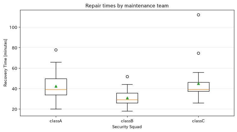
classA	18	39.0264	31.2222
classB	18	29.2456	17.6111
classC	18	38.9934	33.6667

	Hvalue	degree of freedom	pvalue	epsilonsquare	determination
0	10.8853	2	0.0043	0.1742	at least1There are differences among the flocks.

Reading the results

Based on the overall p-value and effect size, determine whether the distribution differences between groups can be neglected. Do not immediately consider a group with a longer median as “incompetent.” The configuration of assigned equipment, failure modes, nighttime calls, and parts waiting times may differ. Failure difficulty is stratified, and p-value correction is performed in post-test comparisons after the overall test.

No.059: Kolmogorov–Smirnov Test — Detecting Deviations from Reference Distributions

Meaning in Practice

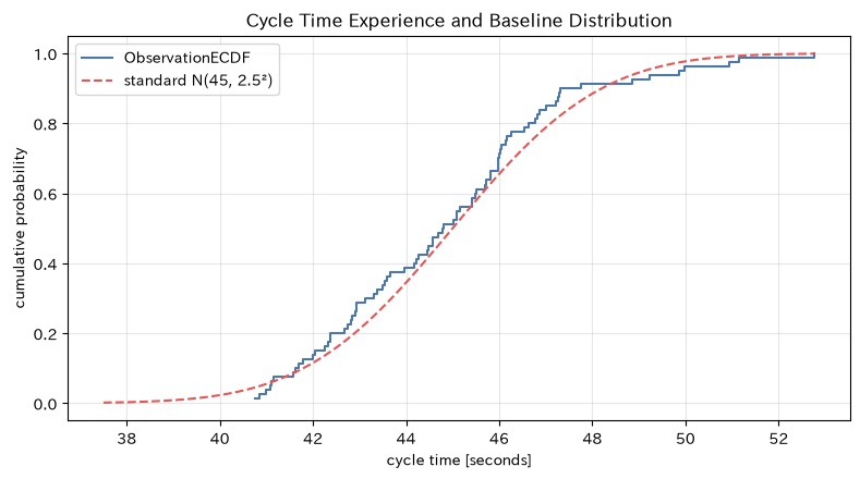
Check that the cycle time matches the fixed reference distribution $N(45, 2.5^2)$ at installation. It captures distortions, hems, and local stagnations across the distribution that can be overlooked by means and standard deviations alone.

Approach to Analysis and Modeling

The statistical measure of the one-sample Kolmogorov–Smirnov test shows the maximum difference between the cumulative $F_n(x)$ experience and the $F_0(x)$ cumulative distribution

$$D=\sup_x\left|F_n(x)-F_0(x)\right|$$

That’s right. Assuming a continuous distribution. The important thing is to Not estimated from this sample the mean and standard deviation of the reference distribution. Using the same data, the p-value of the standard KS test is inappropriate, and Lilliefors-type corrections or bootstrapping are necessary.

Check with Python

target_mu59, target_sd59 = 45.0, 2.5
target_cdf59 = lambda x: stats.norm.cdf(x, loc=target_mu59, scale=target_sd59)
ks59 = stats.kstest(cycle_time, target_cdf59)
x59 = np.sort(cycle_time)
ecdf59 = np.arange(1, len(x59) + 1) / len(x59)
grid59 = np.linspace(min(x59.min(), 37.5), max(x59.max(), 52.5), 300)

display(pd.DataFrame({
    "Sample size": [len(cycle_time)], "specimen mean[seconds]": [cycle_time.mean()],
    "specimen_standard_deviation": [cycle_time.std(ddof=1)], "Benchmark Average": [target_mu59],
    "reference standard deviation": [target_sd59], "KSstatistical quantityD": [ks59.statistic], "pvalue": [ks59.pvalue],
    "determination": ["Differences from the reference distribution" if ks59.pvalue < ALPHA else "Unable to confirm the difference,"]
}))

fig, ax = plt.subplots()
ax.step(x59, ecdf59, where="post", label="ObservationECDF", color="#4C78A8")
ax.plot(grid59, stats.norm.cdf(grid59, target_mu59, target_sd59),
        label="standard N(45, 2.5²)", color="#E45756", linestyle="--")
ax.set_title("Cycle Time Experience and Baseline Distribution")
ax.set_xlabel("cycle time [seconds]")
ax.set_ylabel("cumulative probability")
ax.grid(alpha=0.3)
ax.legend()
plt.tight_layout()
plt.show()

	Sample size	specimen mean[seconds]	specimen_standard_deviation	Benchmark Average	reference standard deviation	KSstatistical quantityD	pvalue	determination
0	80	44.8608	2.5536	45.0	2.5	0.0838	0.5986	Unable to confirm the difference,

Reading the results

The maximum vertical difference between the ECDF and the reference CDF is the KS statistic. In a long distribution on the right side like this, not only averages but also slow cycle accumulations can be detected. If there are discrepancies, we suspect a mix of short-term stops, waiting for material supplies, or work interventions. The KS test does not specify the location or cause of the difference, so it checks it with quantile differences and logs.

No.060: Ljung–Box Test — Examining the Autocorrelation of Furnace Temperature Model Residuals

Meaning in Practice

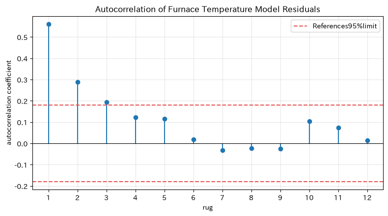
Check whether the residuals of the furnace temperature prediction model are not continuous in the time direction. If the residual remains autocorrelated, the model may not capture thermal inertia or control periods, leading to repeated false alarms in anomaly judgments and underestimation of prediction intervals.

Approach to Analysis and Modeling

The Ljung–Box test collectively tests autocorrelation from Lag 1 to $h$.

$$Q=n(n+2)\sum_{k=1}^{h}\frac{\hat{\rho}_k^2}{n-k}$$

The null hypothesis is that all autocorrelations up to the specified lag are zero. $Q$ approximately follows the chi-square distribution. When applying to estimated model residuals such as ARIMA, the degrees of freedom need to be subtracted from the estimated number of AR/MA parameters. Here, we will set the degrees of freedom as the fixed prediction model residual for explanation, $h$.

Check with Python

def ljung_box(x, max_lag):
    x = np.asarray(x) - np.mean(x)
    n = len(x)
    denominator = np.dot(x, x)
    acf = np.array([np.dot(x[k:], x[:-k]) / denominator for k in range(1, max_lag + 1)])
    lags = np.arange(1, max_lag + 1)
    q_values = n * (n + 2) * np.cumsum(acf ** 2 / (n - lags))
    p_values = stats.chi2.sf(q_values, df=lags)
    return lags, acf, q_values, p_values

lags60, acf60, q60, p60 = ljung_box(temp_residual, max_lag=12)
result60 = pd.DataFrame({"rug": lags60, "autocorrelation": acf60,
                         "AccumulateQvalue": q60, "pvalue": p60})
display(result60.round(4))
display(pd.DataFrame({"Evaluation lag": [12], "Ljung-Box Q": [q60[-1]], "pvalue": [p60[-1]],
                      "determination": ["Autocorrelation" if p60[-1] < ALPHA else "Unable to confirm autocorrelation"]}))

fig, ax = plt.subplots()
ax.stem(lags60, acf60, basefmt=" ")
bound60 = 1.96 / np.sqrt(len(temp_residual))
ax.axhline(bound60, color="#E45756", linestyle="--", label="References95%limit")
ax.axhline(-bound60, color="#E45756", linestyle="--")
ax.axhline(0, color="black", linewidth=0.8)
ax.set_title("Autocorrelation of Furnace Temperature Model Residuals")
ax.set_xlabel("rug")
ax.set_ylabel("autocorrelation coefficient")
ax.set_xticks(lags60)
ax.grid(alpha=0.3)
ax.legend()
plt.tight_layout()
plt.show()

	rug	autocorrelation	AccumulateQvalue	pvalue
0	1	0.5605	38.6467	0.0
1	2	0.2884	48.9647	0.0
2	3	0.1936	53.6523	0.0
3	4	0.1218	55.5232	0.0
4	5	0.1156	57.2235	0.0
5	6	0.0181	57.2658	0.0
6	7	-0.0316	57.3950	0.0
7	8	-0.0229	57.4635	0.0
8	9	-0.0249	57.5455	0.0
9	10	0.1029	58.9560	0.0
10	11	0.0745	59.7013	0.0
11	12	0.0141	59.7282	0.0

	Evaluation lag	Ljung-Box Q	pvalue	determination
0	12	59.7282	2.5300e-08	Autocorrelation

Reading the results

If positive autocorrelation is observed in small lags and the p-value up to lug 12 is small, it is considered difficult to regard the residual as independent noise. Thermal inertia of the furnace, setting change history, transport cycle, sensor smoothing, and other factors are incorporated into feature or time-series models. The Ljung–Box test does not indicate “which model is correct,” but rather that the residual leaves an unexplained time structure.

Practical Implications Seen Through Target Exercise

The 10 types of tests are assigned roles depending on the questions they cover.

• When asking for means, the method changes depending on group 1, correspondence, independent group 2, or group 3 or more
• For category ratios, if the expected power is sufficient, chi-square is a candidate; if the small sample is 2×2 table, Fisher is a candidate
• For continuous quantities with strong outliers or distortions, ranking tests are strong, but care must be taken when interpreting the test subject
• To test not only mean and median values but also the entire distribution, use the KS test; to test independence of time series, use the Ljung–Box test
• The p-value is neither the magnitude of the effect nor the probability that the null hypothesis is correct. Include differences, confidence intervals, and effect sizes together
• “No significant difference” is not proof of equivalence. If you want to demonstrate equivalence, design an equivalence test with tolerance

Most importantly, rather than looking at the data and then choosing the most convenient test, first define on-site decision-making, comparative units, and minimum importance differences.

What is necessary for practical implementation

1. Check the measurement system: Evaluate calibration, resolution, measure-based error, and under-measurement or rounding
2. Aligning the analysis units: Decide whether the product can be considered an independent specimen or should be measured by lot or equipment
3. Leave a plan ahead: Record hypotheses, one-sided or two-sided, significance levels, required sample size, and exclusion rules
4. Set practical thresholds: Set the minimum effect required for adoption in addition to statistical significance
5. Managing Confusion: Randomize and stratify by type, material, worker, time of day, and equipment condition
6. Addressing Multiplicity: When comparing many indicators, groups, or periods, narrow down and adjust the main hypothesis.
7. Connect to continuous monitoring: Don’t stop at a single test—track sustained effectiveness with management charts and KPIs.
8. make reproducible: Manage source data, code, environment, execution date, analyst, and judgment

Changes related to safety, regulations, and customer assurance are not automatically approved based solely on p-values, but are combined with FMEA, process capability, change management, and expert reviews.

Conclusion

In No.051 to No.060, representative comparative issues in manufacturing sites were identified using t-tests, corresponding t-tests, Welch tests, chi-squares tests, Fisher’s exact tests, ANOVAs, Mann–Whitney tests, Kruskal–Wallis tests, Kolmogorov–Smirnov tests, and Ljung–Box tests.

To turn test results into decision-making, it is more important to align questions and data structures than to API the method. By compiling p-values, effect sizes, confidence intervals, graphs, and on-site tolerances into a single judgment data, you can avoid overestimating improvement effects and minimize oversights.

Consultations for Corporations

At Surikoubo, we support quality data analysis, experimental planning, verification of process improvement effects, anomaly detection, demand, inventory, and production planning, as well as in-house data talent development in manufacturing.

From stages such as “I can’t choose a certification that fits on-site data,” “Significant differences emerged but don’t lead to management decisions,” or “I want to migrate Excel analysis to reproducible Python operations,” we can consult with you from problem organization, analysis design, implementation, to operational firming.

📩 Contact Us: surikobo.co.jp/contact
Please feel free to consult us first.