
100 Exercises / Probability Statistics / Probability & Statistics: Python 100 Exercises
Connecting Uncertainty to Judgments on Equipment, Inventory, and Production Capacity: 10 Exercises on Manufacturing Simulations
Connecting Uncertainty to Judgments on Equipment, Inventory, and Production Capacity: 10 Exercises on Manufacturing Simulations
On the manufacturing floor, even if average demand, standard time, and mean interval between failures are known, it is unclear when stockouts, stagnations, and stoppages will overlap. In this article, we will implement Monte Carlo integrals, queues, inventory, failures, agents, Markov chains, discrete events, Brownian movements, stochastic differential equations, digital twins using Python as the subject of a fictional precision parts factory.
The goal is not to line up simulation methods, but to lead to decisions such as “whether to increase inspection capacity,” “how many safety stock to maintain,” “when to conduct preventive maintenance,” and “how to compare capital investment proposals.” The target is a probability and statistics Python implementation No.091〜No.100 with 100 Exercises.
[!NOTE] This material is a notebook previously used by Surikoubo (or personally by the representative, Kazuyama), and has been reconstructed, edited, and published with the company’s permission.
All data listed is fictional and has no relation whatsoever to real companies, factories, or figures.
Introduction: Practical Challenges in Manufacturing Covered in This Article
At a fictional precision pump parts factory, we are reviewing production plans and capital investments for the next quarter. Orders fluctuate daily, parts replenishment takes time, and equipment frequently fails. Furthermore, post-processing inspections have become a bottleneck, and work-in-progress stagnation is putting pressure on delivery deadlines.
These issues cannot be judged by average values alone. It is necessary to reproduce multiple uncertainties over time and compare KPI distributions, deterioration conditions, and trade-offs between measures. In this article, we start with a small, auditable model and finally integrate it into a simple digital twin updated with field data.
Common situations on site
- Although average processing capacity exceeds demand, wait times for inspections surge only during busy periods.
- Sets safety stock based on empirical rules and fails to compare out-of-stock losses with holding costs.
- Only the mean interval between failures is used, without considering equipment deterioration or preventive maintenance timing
- While improvement proposals for each process can be evaluated, the overall lead time effect of the factory is not visible.
- Even if simulation figures deviate from on-site performance, the update method and responsible person have not been decided.
Simulations do not predict the future at all points. It is decision support for comparing the distribution of outcomes for each alternative on the same standard under uncertain assumptions.
Why is this issue so difficult to judge?
Demand, processing time, failures, and replenishment lead times are random variables, and their effects accumulate over time. Even if average demand is lower than average capacity, if utilization approaches 1, wait times increase nonlinearly. Additionally, measures to reduce out-of-stock rates increase inventory costs, while measures that increase preventive maintenance decrease breakdowns while increasing planned downtime.
The expected value estimated by simulation is generally
It can be expressed as such. However, finite attempts have Monte Carlo errors, and if the input distribution is incorrect, the precise output will also be incorrect. Therefore, not only averages but also quantiles, confidence intervals, sensitivity, reproducibility, and model validity are checked.
Overview of Exercise covered this time
| No. | Theme | Questions in the Manufacturing Industry |
|---|---|---|
| 091 | Monte Carlo integral | Can you estimate expected shortage costs, including demand fluctuations? |
| 092 | Queue simulation | What are the waiting times for full inspections and the rate of SLA exceedance? |
| 093 | Inventory Simulation | How Stockouts and Inventory Costs Change When Ordering Points Are Changed |
| 094 | Failure Simulation | How many days should the preventive maintenance cycle be set? |
| 095 | Agent Simulation | Is dynamic sorting more effective than fixed sorting in products? |
| 096 | Markov chain | Can long-term downtime rates be estimated from equipment condition transitions? |
| 097 | Discrete Event Simulation | Where are the bottlenecks in multi-process lines? |
| 098 | Brownian motion | What is the risk of reaching the sensor drift threshold? |
| 099 | Probability differential equation | Can the mean regression of temperature control and disturbances be expressed simultaneously? |
| 100 | Introduction to Digital Twins | Can improvements be compared from models updated based on actual experience? |
The first half addresses individual uncertainties, the second half expresses dependencies on state, time, and processes, and finally consolidates data updates and scenario comparisons into a single operational loop.
Preparing the Python environment
NumPy performs random numbers and numerical calculations, pandas tables for tables, SciPy for distribution and integration, and matplotlib for visualization. japanize_matplotlib is used only for Japanese label display; seaborn or external data is not used. For reproducibility, the seed for the entire analysis is fixed.
import platform
import heapq
import numpy as np
import pandas as pd
import scipy
from scipy import integrate, stats
import matplotlib
import matplotlib.pyplot as plt
import japanize_matplotlib

SEED = 20260711
rng = np.random.default_rng(SEED)
plt.rcParams["figure.figsize"] = (8, 4.5)
plt.rcParams["axes.unicode_minus"] = False

print(f"Python     : {platform.python_version()}")
print(f"NumPy      : {np.__version__}")
print(f"pandas     : {pd.__version__}")
print(f"SciPy      : {scipy.__version__}")
print(f"Matplotlib : {matplotlib.__version__}")
print(f"random seed: {SEED}")
Python : 3.13.1
NumPy : 2.5.1
pandas : 3.0.3
SciPy : 1.18.0
Matplotlib : 3.11.0
random seed: 20260711Creation of Fictional Data
The target is a precision pump parts factory that operates 8 hours a day, 240 days a year. Generate demand for the past 120 days, inspection arrival intervals, inspection times, equipment status, and furnace temperature in Python. The “observation data” here will also be used later for digital twin updates.
This is because the teaching materials can place the true generation conditions within the code. In practice, we organize missing measurements, stoppages during stoppages, product composition, planned stoppages, and work structures, diagnose distribution assumptions, and then create model inputs.
n_history_days = 120
daily_demand = np.maximum(0, rng.normal(102, 18, n_history_days).round()).astype(int)
inspection_interarrival = rng.exponential(scale=5.2, size=1500)  # minutes
inspection_service = rng.lognormal(mean=np.log(4.4), sigma=0.25, size=1500)  # minutes
equipment_states = rng.choice(["sound", "deterioration", "stop"], size=n_history_days,
                              p=[0.78, 0.17, 0.05])
furnace_temperature = 180 + rng.normal(0, 1.8, n_history_days)

factory_data = pd.DataFrame({
    "item": ["daily demand", "Interval between test arrivals", "Examination Hours", "Facility Condition", "furnace temperature"],
    "Number of observations": [len(daily_demand), len(inspection_interarrival), len(inspection_service),
             len(equipment_states), len(furnace_temperature)],
    "Summary": [f"average {daily_demand.mean():.1f} units/days",
           f"average {inspection_interarrival.mean():.2f} minutes",
           f"average {inspection_service.mean():.2f} minutes",
           f"stop rate {np.mean(equipment_states == 'stop'):.1%}",
           f"average {furnace_temperature.mean():.2f} ℃"],
})
factory_data| item | Number of observations | Summary | |
|---|---|---|---|
| 0 | daily demand | 120 | average 101.7 units/days |
| 1 | Interval between test arrivals | 1500 | average 5.05 minutes |
| 2 | Examination Hours | 1500 | average 4.48 minutes |
| 3 | Facility Condition | 120 | stop rate 5.0% |
| 4 | furnace temperature | 120 | average 179.99 ℃ |
No.091: Monte Carlo Integral — Estimating Expected Loss Due to Excess Demand
Meaning in Practice
When determining Nissan’s capacity, even meeting only average demand can lead to overwhelmed demand and missed orders. Assuming a loss of 4,500 yen per unit for a quantity exceeding capacity , the expected loss is assessed.
Approach to Analysis and Modeling
If demand and loss , the expected loss is
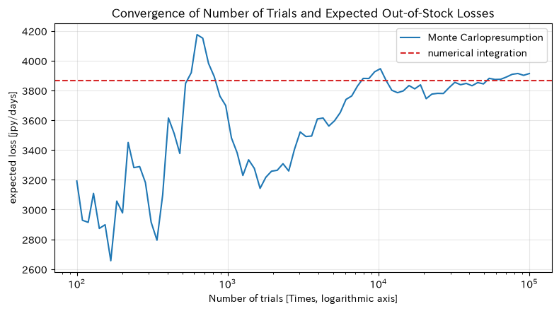
That’s right. In the Monte Carlo method, demand is repeatedly generated to calculate the sample average. Since the estimated standard error decreases at about , it takes about four times the number of attempts to double the accuracy.
Check with Python
mu_d, sigma_d, capacity, penalty = 102, 18, 125, 4500
n_mc = 100_000
mc_demand = rng.normal(mu_d, sigma_d, n_mc)
mc_loss = penalty * np.maximum(mc_demand - capacity, 0)
mc_estimate = mc_loss.mean()
mc_se = mc_loss.std(ddof=1) / np.sqrt(n_mc)

integral_value, _ = integrate.quad(
    lambda d: penalty * (d - capacity) * stats.norm.pdf(d, mu_d, sigma_d),
    capacity, np.inf,
)
mc_table = pd.DataFrame({
    "Methods": ["Monte Carlo", "numerical integration"],
    "expected loss [jpy/days]": [mc_estimate, integral_value],
    "Monte Carlostandard error [jpy]": [mc_se, np.nan],
})
display(mc_table.round(1))

checkpoints = np.unique(np.logspace(2, 5, 80).astype(int))
cumulative_estimates = np.cumsum(mc_loss)[checkpoints - 1] / checkpoints
plt.plot(checkpoints, cumulative_estimates, label="Monte Carlopresumption")
plt.axhline(integral_value, color="tab:red", ls="--", label="numerical integration")
plt.xscale("log")
plt.title("Convergence of Number of Trials and Expected Out-of-Stock Losses")
plt.xlabel("Number of trials [Times, logarithmic axis]")
plt.ylabel("expected loss [jpy/days]")
plt.grid(True, alpha=0.3)
plt.legend()
plt.tight_layout()
plt.show()| Methods | expected loss [jpy/days] | Monte Carlostandard error [jpy] | |
|---|---|---|---|
| 0 | Monte Carlo | 3913.0 | 49.6 |
| 1 | numerical integration | 3865.5 | NaN |
Reading the results
As the number of trials increases, the estimated value approaches the value of the numerical integration. The value of the Monte Carlo method lies not in integrating with just this single variable, but in that it can extend the same thinking to higher-dimensional losses, including product composition, ability decline, and overtime judgments. Not only expected losses but also tail risks such as the 95th percentile are included and compared with capability enhancement costs.
No.092: Queue Simulation — Evaluating Full-Capacity Inspection Delays
Meaning in Practice
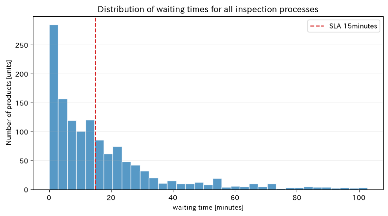
In the inspection process, even if the average processing time is shorter than the arrival interval, differences in arrival and processing can cause waiting times. We look at the average waiting time and the rate of SLA exceedance, which is ‘testing starts within 15 minutes.‘
Approach to Analysis and Modeling
The GI/G/1 type queue where products arrive at a single inspection machine is set as arrival time , start time , and end time
and calculate them sequentially. To approximate steadiness, the rise period is excluded. The higher the utilization rate, the greater the impact of input estimation errors.
Check with Python
def simulate_single_queue(interarrival, service, warmup=200):
    arrival = np.cumsum(interarrival)
    start = np.empty(len(arrival))
    finish = np.empty(len(arrival))
    previous_finish = 0.0
    for i in range(len(arrival)):
        start[i] = max(arrival[i], previous_finish)
        finish[i] = start[i] + service[i]
        previous_finish = finish[i]
    waiting = start - arrival
    return arrival[warmup:], waiting[warmup:], finish[warmup:] - arrival[warmup:]

arrival_q, waiting_q, lead_q = simulate_single_queue(
    inspection_interarrival, inspection_service
)
queue_result = pd.DataFrame({
    "KPI": ["estimated utilization rate", "Average Waiting Time", "waiting time95%point", "15Excess rate"],
    "value": [inspection_service.mean() / inspection_interarrival.mean(),
          waiting_q.mean(), np.quantile(waiting_q, 0.95), np.mean(waiting_q > 15)],
    "Unit": ["ratio", "minutes", "minutes", "ratio"],
})
display(queue_result.round(3))

plt.hist(waiting_q, bins=35, alpha=0.75, edgecolor="white")
plt.axvline(15, color="tab:red", ls="--", label="SLA 15minutes")
plt.title("Distribution of waiting times for all inspection processes")
plt.xlabel("waiting time [minutes]")
plt.ylabel("Number of products [units]")
plt.grid(True, axis="y", alpha=0.3)
plt.legend()
plt.tight_layout()
plt.show()| KPI | value | Unit | |
|---|---|---|---|
| 0 | estimated utilization rate | 0.886 | ratio |
| 1 | Average Waiting Time | 16.735 | minutes |
| 2 | waiting time95%point | 58.754 | minutes |
| 3 | 15Excess rate | 0.394 | ratio |
Reading the results
By looking at the 95% score and SLA exceedance rate in addition to the average, you can understand customer impact during busy times. The distribution of wait times is long to the right, and the average alone hides the long stagnation. Before deciding on capacity additions, the model reflects the time of category processing, arrangement, breaks, re-inspections, and arrival time zones to confirm reproducibility with the actual distribution.
No.093: Inventory Simulation — Comparing Order Points with Out-of-Stock/Holding Costs
Meaning in Practice
Increasing safety stock reduces shortages but raises storage space, funds, and the risk of obsolescence. Candidates for order points are compared within the same demand series, and both service rate and total cost are used to determine the results.
Approach to Analysis and Modeling
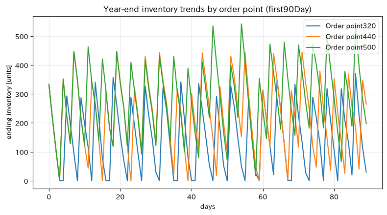
If the inventory position falls below the order point , a fixed quantity is ordered, and the method of receiving goods four days later is reproduced daily. Costs consist of holding costs and penalties for unmet demand. Using common random numbers among candidates allows comparison of policy differences by suppressing coincidence differences in demand series.
Check with Python
def simulate_inventory(demand, reorder_point, order_qty=420, lead_time=4,
                       initial_stock=420, holding_cost=35, shortage_cost=1800):
    on_hand = initial_stock
    pipeline = []
    rows = []
    for day, d in enumerate(demand):
        arrivals = sum(q for due, q in pipeline if due == day)
        pipeline = [(due, q) for due, q in pipeline if due > day]
        on_hand += arrivals
        shipped = min(on_hand, d)
        shortage = d - shipped
        on_hand -= shipped
        position = on_hand + sum(q for _, q in pipeline)
        if position <= reorder_point:
            pipeline.append((day + lead_time, order_qty))
        rows.append((day, d, arrivals, shipped, shortage, on_hand))
    df = pd.DataFrame(rows, columns=["days", "need", "arrival", "Shipping", "missing item", "ending inventory"])
    cost = holding_cost * df["ending inventory"].sum() + shortage_cost * df["missing item"].sum()
    return df, cost

inventory_demand = np.maximum(0, rng.normal(102, 18, 365).round()).astype(int)
inventory_results = []
inventory_paths = {}
for s in [320, 380, 440, 500]:
    path, cost = simulate_inventory(inventory_demand, s)
    inventory_paths[s] = path
    inventory_results.append({
        "Order point": s,
        "sufficiency rate": path["Shipping"].sum() / path["need"].sum(),
        "Average ending inventory": path["ending inventory"].mean(),
        "Quantity of Items Missing": path["missing item"].sum(),
        "Total annual cost [jpy]": cost,
    })
inventory_table = pd.DataFrame(inventory_results)
display(inventory_table.round({"sufficiency rate": 4, "Average ending inventory": 1}))

for s in [320, 440, 500]:
    plt.plot(inventory_paths[s]["days"][:90], inventory_paths[s]["ending inventory"][:90],
             label=f"Order point{s}")
plt.title("Year-end inventory trends by order point (first90Day)")
plt.xlabel("days")
plt.ylabel("ending inventory [units]")
plt.grid(True, alpha=0.3)
plt.legend()
plt.tight_layout()
plt.show()| Order point | sufficiency rate | Average ending inventory | Quantity of Items Missing | Total annual cost [jpy] | |
|---|---|---|---|---|---|
| 0 | 320 | 0.8914 | 150.2 | 4123 | 9339995 |
| 1 | 380 | 0.9824 | 179.9 | 668 | 3500500 |
| 2 | 440 | 0.9980 | 233.5 | 75 | 3117595 |
| 3 | 500 | 1.0000 | 289.6 | 0 | 3699325 |
Reading the results
Generally, the higher the order point, the better the fulfillment rate becomes, but the average inventory and holding costs increase. The minimum cost proposal in the table is a conclusion based on the set shortage unit price and holding unit price, and is not an absolute solution. In practice, we add fluctuations in lead time itself, minimum order quantities, storage constraints for multiple items, backorders, and demand at the time of stopping, and also check the sensitivity of cost parameters.
No.094: Failure Simulation — Designing Preventive Maintenance Cycles
Meaning in Practice
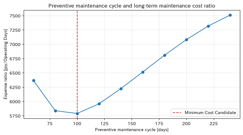
When equipment deteriorates and failure rates increase, it is important to balance post-repair maintenance after failure with preventive maintenance that stops early. Compare long-term expense ratios for each preventive replacement cycle.
Approach to Analysis and Modeling
Lifetime is taken as the Weibull distribution, and the shape parameter represents aging deterioration. If the failure occurs before cycle , repair costs are charged; if not, preventive maintenance costs are charged at . generating multiple cycles of the update process,
This is how it will be evaluated. Each cycle generates a lifetime from the same uniform random number, minimizing variation in comparison.
Check with Python
shape, scale = 2.2, 170.0
n_cycles = 80_000
u_life = rng.random(n_cycles)
lifetimes = scale * (-np.log(1 - u_life)) ** (1 / shape)

maintenance_results = []
for tau in np.arange(60, 241, 20):
    failed = lifetimes < tau
    cycle_length = np.minimum(lifetimes, tau)
    cycle_cost = np.where(failed, 1_200_000, 280_000)
    maintenance_results.append({
        "Preventive maintenance cycle [days]": tau,
        "Probability of failure within the cycle": failed.mean(),
        "Expense ratio [jpy/Operating Days]": cycle_cost.sum() / cycle_length.sum(),
    })
maintenance_table = pd.DataFrame(maintenance_results)
best_tau = maintenance_table.loc[maintenance_table["Expense ratio [jpy/Operating Days]"].idxmin()]
display(maintenance_table.round(2))
print(f"Minimum cost candidate cycle: {best_tau['Preventive maintenance cycle [days]']:.0f} days")

plt.plot(maintenance_table["Preventive maintenance cycle [days]"],
         maintenance_table["Expense ratio [jpy/Operating Days]"], marker="o")
plt.axvline(best_tau["Preventive maintenance cycle [days]"], color="tab:red", ls="--", label="Minimum Cost Candidate")
plt.title("Preventive maintenance cycle and long-term maintenance cost ratio")
plt.xlabel("Preventive maintenance cycle [days]")
plt.ylabel("Expense ratio [jpy/Operating Days]")
plt.grid(True, alpha=0.3)
plt.legend()
plt.tight_layout()
plt.show()| Preventive maintenance cycle [days] | Probability of failure within the cycle | Expense ratio [jpy/Operating Days] | |
|---|---|---|---|
| 0 | 60 | 0.10 | 6365.89 |
| 1 | 80 | 0.17 | 5837.04 |
| 2 | 100 | 0.27 | 5788.45 |
| 3 | 120 | 0.37 | 5957.85 |
| 4 | 140 | 0.48 | 6222.70 |
| 5 | 160 | 0.58 | 6513.43 |
| 6 | 180 | 0.68 | 6807.53 |
| 7 | 200 | 0.76 | 7079.27 |
| 8 | 220 | 0.83 | 7317.14 |
| 9 | 240 | 0.88 | 7509.18 |
Minimum cost candidate cycle: 100 days
Reading the results
If the cycle is too short, preventive maintenance costs increase, and if it is too long, expensive breakdowns increase, so the cost ratio is the lowest in between. This cycle depends on the Weibull assumption and cost setting. If quality leakage, safety, delivery times, or chain stoppages due to failures cannot be realized, not only should the cost be minimized, but there should also be upper limits on the probability of failure.
No.095: Agent Simulation — Comparing Dynamic Distribution by Product
Meaning in Practice
When products are distributed to parallel equipment in fixed proportions, coincidental differences in processing time can cause congestion on only one side. Compare the strategies for selecting equipment that completes the process quickly upon arrival as the decision-maker (agent) for each product.
Approach to Analysis and Modeling
Product agents have their own arrival times and their own processing times. In fixed methods, equipment is selected alternately, while in dynamic measures, the current scheduled completion time for each piece of equipment is checked and the side with the earliest expected completion is chosen. A characteristic of the agent model is that the lead time distribution across the entire factory arises from local rules.
Check with Python
def simulate_routing(arrivals, service_a, service_b, policy):
    available = np.zeros(2)
    records = []
    for i, arrival in enumerate(arrivals):
        service = np.array([service_a[i], service_b[i]])
        if policy == "Fixed alternation":
            machine = i % 2
        else:
            predicted_finish = np.maximum(arrival, available) + service
            machine = int(np.argmin(predicted_finish))
        start = max(arrival, available[machine])
        finish = start + service[machine]
        available[machine] = finish
        records.append((i, arrival, machine, start, finish, finish - arrival))
    return pd.DataFrame(records, columns=["Products", "Arrival", "equipment", "start", "completed", "lead time"])

n_agents = 1200
agent_arrivals = np.cumsum(rng.exponential(2.15, n_agents))
service_a = rng.lognormal(np.log(3.7), 0.28, n_agents)
service_b = rng.lognormal(np.log(4.1), 0.22, n_agents)
routing_tables = {
    policy: simulate_routing(agent_arrivals, service_a, service_b, policy)
    for policy in ["Fixed alternation", "Shortest completion"]
}
routing_result = pd.DataFrame([
    {"policy": policy, "Average lead time [minutes]": df["lead time"].mean(),
     "95%point [minutes]": df["lead time"].quantile(0.95),
     "equipmentAdistribution rate": np.mean(df["equipment"] == 0)}
    for policy, df in routing_tables.items()
])
display(routing_result.round(3))

for policy, df in routing_tables.items():
    plt.hist(df["lead time"], bins=35, density=True, alpha=0.5, label=policy)
plt.title("Product Lead Time Distribution by Distribution Method")
plt.xlabel("lead time [minutes]")
plt.ylabel("probability density")
plt.grid(True, axis="y", alpha=0.3)
plt.legend()
plt.tight_layout()
plt.show()| policy | Average lead time [minutes] | 95%point [minutes] | equipmentAdistribution rate | |
|---|---|---|---|---|
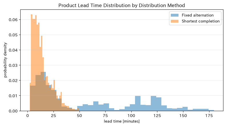
| 0 | Fixed alternation | 55.83 | 141.602 | 0.500 |
| 1 | Shortest completion | 13.81 | 32.225 | 0.527 |
Reading the results
The shortest completion strategy can take advantage of congestion and speed differences between facilities, and sometimes lower the mean lead time or upper quantile compared to fixed alternating periods. However, on-site, you cannot ignore product type, jigs, tools, arrangements, operator qualifications, and transport distance. The more complex the rules are added, the harder it becomes to verify, so we also design explainability for measures and manual operation during failures.
No.096: Markov Chain — Estimating Long-Term Shutdown Rate Based on Equipment Condition
Meaning in Practice
By managing equipment daily in a state of “healthy, deteriorated, and stopped,” you can express the risk of progressing from deterioration to shutdown and the possibility of recovery after repairs, rather than just the number of failures. We calculate the long-term state composition and the future distribution from the current state.
Approach to Analysis and Modeling
The element of transition matrix is the probability that if today is state , the next day will be state . The state distribution is
and the stationary distribution satisfies . Be careful of the assumption that the future depends solely on the current state and does not specify the length of stay.
Check with Python
state_names = np.array(["sound", "deterioration", "stop"])
P = np.array([
    [0.91, 0.08, 0.01],
    [0.24, 0.66, 0.10],
    [0.55, 0.15, 0.30],
])

eigenvalues, eigenvectors = np.linalg.eig(P.T)
stationary = np.real(eigenvectors[:, np.argmin(np.abs(eigenvalues - 1))])
stationary = stationary / stationary.sum()

prob = np.array([0.0, 1.0, 0.0])  # It is now deteriorating
state_history = [prob.copy()]
for _ in range(30):
    prob = prob @ P
    state_history.append(prob.copy())
state_history = np.array(state_history)

display(pd.DataFrame(P, index=state_names, columns=state_names).round(2))
display(pd.DataFrame({"Condition": state_names, "steady probability": stationary}).round(4))

for i, state in enumerate(state_names):
    plt.plot(np.arange(31), state_history[:, i], label=state)
plt.axhline(stationary[2], color="tab:red", ls=":", label="steady stop rate")
plt.title("Current Trends in Equipment Condition Probabilities Starting from 'Deterioration'")
plt.xlabel("Number of days elapsed [days]")
plt.ylabel("State probability")
plt.grid(True, alpha=0.3)
plt.legend()
plt.tight_layout()
plt.show()| sound | deterioration | stop | |
|---|---|---|---|
| sound | 0.91 | 0.08 | 0.01 |
| deterioration | 0.24 | 0.66 | 0.10 |
| stop | 0.55 | 0.15 | 0.30 |
| Condition | steady probability | |
|---|---|---|
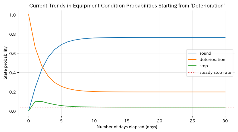
| 0 | sound | 0.7640 |
| 1 | deterioration | 0.1970 |
| 2 | stop | 0.0391 |
Reading the results
Even if the current state is deteriorating, as days pass, the initial state effect diminishes and the state probability approaches a steady distribution. The steady-state downtime rate is an input for long-term capacity planning, but for equipment whose failure rate changes the next day based on “how many days it has been in a deteriorating state,” simple Markov characteristics are insufficient. In such cases, the state is subdivided, or the Semi-Markov model or the survival time model is considered.
No.097: Discrete Event Simulation — Identifying Bottlenecks in Multi-Process Lines
Meaning in Practice
When pressing, machining, and inspection are connected in series, the average time for each process alone cannot assess the overall lead time of the factory. Only the events of product arrival, processing start, and processing completion advance the time, and wait times for each process are measured.
Approach to Analysis and Modeling
In discrete event simulation, the clock advances to the next event time without updating all states in fixed increments. Here, the available times for each process are managed, and three series processes are passed through each product. The inter-process buffer is unlimited, with no failures or overtaking, making it a simplified solution.
Check with Python
def simulate_serial_line(arrivals, service_matrix, machine_counts=(1, 1, 1)):
    machine_available = [np.zeros(m) for m in machine_counts]
    records = []
    for job, arrival in enumerate(arrivals):
        ready = arrival
        for process in range(service_matrix.shape[1]):
            machine = int(np.argmin(machine_available[process]))
            start = max(ready, machine_available[process][machine])
            finish = start + service_matrix[job, process]
            records.append((job, process, machine, ready, start, finish, start - ready))
            machine_available[process][machine] = finish
            ready = finish
    return pd.DataFrame(records, columns=["Products", "Project", "equipment", "Arrival", "start", "completed", "wait"])

n_jobs = 900
line_arrivals = np.cumsum(rng.exponential(4.8, n_jobs))
service_matrix = np.column_stack([
    rng.lognormal(np.log(3.2), 0.18, n_jobs),
    rng.lognormal(np.log(4.3), 0.25, n_jobs),
    rng.lognormal(np.log(3.8), 0.20, n_jobs),
])
line_result = simulate_serial_line(line_arrivals, service_matrix)
process_names = {0: "Press", 1: "processing", 2: "inspection"}
process_kpi = line_result.groupby("Project").agg(
    average_waiting_time=("wait", "mean"),
    value_95_waiting_points=("wait", lambda x: x.quantile(0.95)),
).reset_index()
process_kpi["Project Name"] = process_kpi["Project"].map(process_names)
process_kpi["Utilization Estimate"] = [
    service_matrix[:, p].sum() / (line_result["completed"].max() - line_arrivals.min())
    for p in range(3)
]
display(process_kpi[["Project Name", "average_waiting_time", "value_95_waiting_points", "Utilization Estimate"]].round(3))

plot_data = process_kpi.set_index("Project Name")
plot_data["average_waiting_time"].plot(kind="bar", color="tab:blue", alpha=0.75)
plt.title("Average Waiting Time by Process in Series Production Lines")
plt.xlabel("Project")
plt.ylabel("Average Waiting Time [minutes]")
plt.grid(True, axis="y", alpha=0.3)
plt.xticks(rotation=0)
plt.tight_layout()
plt.show()| Project Name | average_waiting_time | wait95point by bit | Utilization Estimate | |
|---|---|---|---|---|
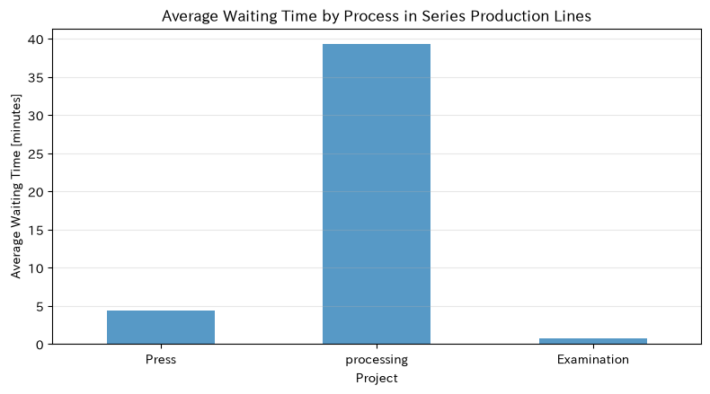
| 0 | Press | 4.324 | 15.194 | 0.695 |
| 1 | processing | 39.328 | 92.109 | 0.962 |
| 2 | inspection | 0.742 | 3.100 | 0.822 |
Reading the results
If the utilization rate and waiting times in the processing process are high, that becomes a potential bottleneck for the entire line. Even if you only speed up processes other than bottlenecks, the overall lead time improvement is limited. The operational model includes finite buffers, blocking, setup, failure, work calendars, and lot transport, and separately verifies process performance and product-specific lead times.
No.098: Brownian Motion — Examining the Risk of Sensor Drift Threshold Reaching
Meaning in Practice
If the zero point of the measuring instrument accumulates small disturbances and shifts, uncertainty will increase over time, even if the mean is zero. Estimate the probability of reaching the calibration tolerance and create candidate inspection cycles.
Approach to Analysis and Modeling
The standard Brownian motion has independent increments and is . If the drift amount is , the variance is and proportional to the time. Here, daily increments are generated to evaluate multiple paths and initial threshold reach.
Check with Python
n_paths, n_days, sigma_sensor, limit = 4000, 60, 0.018, 0.12
increments = rng.normal(0, sigma_sensor, size=(n_paths, n_days))
brownian_paths = np.column_stack([np.zeros(n_paths), np.cumsum(increments, axis=1)])
crossed = np.any(np.abs(brownian_paths[:, 1:]) >= limit, axis=1)
first_crossing = np.where(
    crossed, np.argmax(np.abs(brownian_paths[:, 1:]) >= limit, axis=1) + 1, np.nan
)
brownian_table = pd.DataFrame({
    "KPI": ["60Threshold Reach Within Days", "Median first arrival date of the route reached", "60Day Standard Deviation"],
    "value": [crossed.mean(), np.nanmedian(first_crossing), brownian_paths[:, -1].std(ddof=1)],
    "Unit": ["ratio", "days", "mm"],
})
display(brownian_table.round(4))

days = np.arange(n_days + 1)
for path in brownian_paths[:20]:
    plt.plot(days, path, alpha=0.35, lw=0.9)
plt.axhline(limit, color="tab:red", ls="--", label="Calibration tolerance")
plt.axhline(-limit, color="tab:red", ls="--")
plt.title("Sensor drift pathways represented by Brownian motion")
plt.xlabel("Number of days elapsed [days]")
plt.ylabel("zero-point drift [mm]")
plt.grid(True, alpha=0.3)
plt.legend()
plt.tight_layout()
plt.show()| KPI | value | Unit | |
|---|---|---|---|
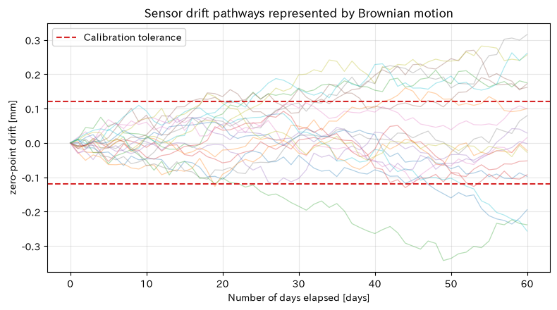
| 0 | 60Threshold Reach Within Days | 0.7058 | ratio |
| 1 | Median first arrival date of the route reached | 29.0000 | days |
| 2 | 60Day Standard Deviation | 0.1406 | mm |
Reading the results
While the direction of each path cannot be predicted, the distribution expands over time, allowing you to evaluate the probability of reaching the acceptable range. When determining the inspection cycle based on these results, the missed losses and calibration costs are compared. Since actual sensors may have mean regression, temperature dependence, step changes, and degradation tendencies, Brownian motion is only used when residual independence and variance growth align with the actual results.
No.099: Stochastic Differential Equations — Reproducing Mean Regression and Disturbances of Furnace Temperature
Meaning in Practice
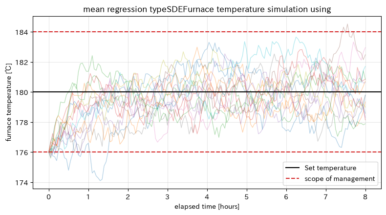
The furnace temperature fluctuates due to disturbances but returns to the set value through control. This “return force” is represented simultaneously with random disturbances, and the probability of temperature exceeding the standard and the effects of control enhancement are compared.
Approach to Analysis and Modeling
The Ornstein–Uhlenbeck process
That’s how it is placed. is the set value, is the speed of returning to the average, and is the disturbance intensity. In the Euler–Maruyama method,
Discretize it with this method. Stability checks with different intervals are necessary.
Check with Python
def simulate_ou(n_paths, hours, dt, x0, mu, theta, sigma, random_generator):
    n_steps = int(hours / dt)
    x = np.empty((n_paths, n_steps + 1))
    x[:, 0] = x0
    z = random_generator.normal(size=(n_paths, n_steps))
    for t in range(n_steps):
        x[:, t + 1] = (x[:, t] + theta * (mu - x[:, t]) * dt
                       + sigma * np.sqrt(dt) * z[:, t])
    return x

dt, hours = 0.05, 8
ou_paths = simulate_ou(3000, hours, dt, x0=176, mu=180,
                       theta=1.1, sigma=2.0, random_generator=rng)
time_grid = np.arange(ou_paths.shape[1]) * dt
out_of_spec = np.mean((ou_paths < 176) | (ou_paths > 184))
ou_table = pd.DataFrame({
    "KPI": ["8Average temperature after time", "8post-time standard deviation", "Non-standard ratio at all times"],
    "value": [ou_paths[:, -1].mean(), ou_paths[:, -1].std(ddof=1), out_of_spec],
    "Unit": ["℃", "℃", "ratio"],
})
display(ou_table.round(3))

for path in ou_paths[:15]:
    plt.plot(time_grid, path, alpha=0.35, lw=0.9)
plt.axhline(180, color="black", lw=1.5, label="Set temperature")
plt.axhline(184, color="tab:red", ls="--", label="scope of management")
plt.axhline(176, color="tab:red", ls="--")
plt.title("mean regression typeSDEFurnace temperature simulation using")
plt.xlabel("elapsed time [hours]")
plt.ylabel("furnace temperature [℃]")
plt.grid(True, alpha=0.3)
plt.legend()
plt.tight_layout()
plt.show()| KPI | value | Unit | |
|---|---|---|---|
| 0 | 8Average temperature after time | 179.997 | ℃ |
| 1 | 8post-time standard deviation | 1.372 | ℃ |
| 2 | Non-standard ratio at all times | 0.015 | ratio |
Reading the results
Even if the initial temperature is lower than the set value, the path average fluctuates due to disturbances as it approaches the set value. The non-standard ratio is determined by the combination of control strength and disturbance strength, allowing comparison of control modification proposals. However, we do not confuse observation noise with process disturbances; instead, we check reproducibility over estimated periods, diagnose residuals, and check out-of-model behavior during abnormalities.
No.100: Introduction to Digital Twins — Updating with Achievements and Comparing Capital Investment Proposals
Meaning in Practice
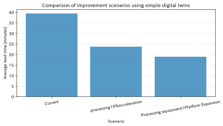
A digital twin is not a 3D display itself, but a mechanism that continuously connects the site’s conditions, data, and models, and is used for scenario comparison and feedback. Here, we update arrival and process times based on actual results, compare current lines, processing speeds, and equipment expansion.
Approach to Analysis and Modeling
A simple twin is structured as a loop: (1) observation, (2) parameter updates, (3) simulation, (4) KPI comparison, and (5) re-verification based on differences from actual results. Inputs are not only point estimation but also stored as distributions. Equal virtual demand and processing time are shared across measures to compare differences.
Check with Python
# Update twin input from observational data (simple experiential distribution for explanation)
observed_interarrival = rng.exponential(4.9, 600)
observed_service = np.column_stack([
    rng.lognormal(np.log(3.3), 0.18, 600),
    rng.lognormal(np.log(4.4), 0.25, 600),
    rng.lognormal(np.log(3.7), 0.20, 600),
])

n_twin_jobs = 1600
twin_arrivals = np.cumsum(rng.choice(observed_interarrival, n_twin_jobs, replace=True))
twin_service = np.column_stack([
    rng.choice(observed_service[:, p], n_twin_jobs, replace=True) for p in range(3)
])

twin_scenarios = {
    "Current": ((1, 1, 1), twin_service.copy()),
    "processing10%acceleration": ((1, 1, 1), twin_service * np.array([1.0, 0.9, 1.0])),
    "Processing equipment1Platform Expansion": ((1, 2, 1), twin_service.copy()),
}
twin_results = []
for scenario, (counts, services) in twin_scenarios.items():
    result = simulate_serial_line(twin_arrivals, services, machine_counts=counts)
    completion = result.groupby("Products")["completed"].max()
    lead_time = completion.to_numpy() - twin_arrivals
    makespan = completion.max() - twin_arrivals.min()
    twin_results.append({
        "Scenario": scenario,
        "Average lead time [minutes]": lead_time.mean(),
        "95%point [minutes]": np.quantile(lead_time, 0.95),
        "throughput [units/8hours]": n_twin_jobs / makespan * 480,
    })
twin_table = pd.DataFrame(twin_results)
twin_table["averageLTimprovement rate"] = 1 - twin_table["Average lead time [minutes]"] / twin_table.loc[0, "Average lead time [minutes]"]
display(twin_table.round(3))

x = np.arange(len(twin_table))
plt.bar(x, twin_table["Average lead time [minutes]"], alpha=0.75)
plt.xticks(x, twin_table["Scenario"], rotation=10)
plt.title("Comparison of improvement scenarios using simple digital twins")
plt.xlabel("Scenario")
plt.ylabel("Average lead time [minutes]")
plt.grid(True, axis="y", alpha=0.3)
plt.tight_layout()
plt.show()| Scenario | Average lead time [minutes] | 95%point [minutes] | throughput [units/8hours] | averageLTimprovement rate | |
|---|---|---|---|---|---|
| 0 | Current | 39.323 | 78.132 | 98.509 | 0.000 |
| 1 | processing10%acceleration | 23.699 | 44.927 | 98.517 | 0.397 |
| 2 | Processing equipment1Platform Expansion | 18.906 | 34.792 | 98.509 | 0.519 |
Reading the results
By comparing the average, 95% points, and throughput for each improvement proposal, you can see the difference in the impact of localized processing time reductions and equipment expansion on the entire line. However, investment decisions require considering equipment costs, maintenance personnel, installation space, and constraints on upstream and downstream processes. Twins are not created once and are not the end; the core operation is to monitor errors between predictions and actual performance, update input distributions, rules, and versions with approval.
Practical Implications Seen Through Target Exercise
- Compare by distribution, not average: In addition to average wait time and expected cost, showing 95% points, SLA exceedance rate, and threshold reach rate helps assess risks during busy periods or abnormal periods.
- Use the same random number conditions for comparison.: By using common demand, lifespan, and processing time, it becomes easier to identify policy differences rather than accidental differences.
- Model granularity aligns with decision-making: For inventory management, we express only the necessary time, entity, and condition—for daily inventory management, for transport or processing, event units; for equipment health, state transitions.
- Don’t overestimate improvements beyond bottlenecks: Always check whether improvements in local KPIs translate into lead times and throughput across the entire line.
- Digital twins include the update process: Practical value only arises when data connection, input estimation, validation, scenario approval, and result monitoring are continuously completed.
The simulation results are prerequisite comparative materials. It is more important to clearly state assumptions, errors, scope of application, and judgment rules than to increase the number of output digits.
What is necessary for practical implementation
- Decision-making andKPIDefinition: Define who, when, and what models to choose, and agree on priorities for cost, delivery time, quality, and safety.
- Maintenance of Time and Status Data: Record arrivals, starts, ends, stops, equipment, varieties, lots, and work calendars with consistent definitions.
- input analysis: Check distribution fit, correlation, time zone, seasonality, cutoffs, and outliers to avoid overconfidence in point estimation.
- VerificationAndValidation: Conduct standalone tests to ensure the code meets specifications, and confirm on-site whether the model reproduces the actual average, quantiles, and stagnation points.
- Sensitivity and Uncertainty Analysis: Check if the conclusion doesn’t reverse when you change inputs, costs, or constraints.
- Operational Governance: Manage model versions, data periods, approvers, update frequency, estimated and actual discrepancies, stop conditions, and switching to manual judgment.
First, we run alongside current operations at the limited line, fix forecasts before decision-making, and accumulate the actual estimate and actual results. We evaluate not only accuracy but also operational KPIs including shortage reduction, delivery deadline compliance, decision time, and on-site load.
Conclusion
From No.091 to No.100, starting with the Monte Carlo integral of expected loss, we implemented queues, inventory, failures, agents, Markov chains, discrete events, Brownian movements, and stochastic differential equations, and finally integrated them into a simple digital twin that updates input with actual data.
The common idea is Represent on-site uncertainty and time dependence with sufficient granularity, compare alternatives under the same conditions, and distribute the resultsKPITranslating to. In practical implementation, it is important to establish operations that define event time, equipment status, product and lot data, and continuously monitor actual estimates before advanced models.
Consultations for Corporations
At Surikoubo, we support everything from production line simulation, inventory and maintenance strategy design, capital investment scenario evaluation, digital twin PoC, Python training, to on-site data infrastructure and operational implementation in manufacturing. You can consult from stages such as “Delivery times are irregular even though average capacity is sufficient,” “I want to compare effects before expanding equipment,” or “I created a simulation but can’t update it on-site.”
📩 Contact Us: surikobo.co.jp/contact
Please feel free to consult us first.