Deciphering Demand Fluctuations and Connecting to Production Planning: 10 Key Steps in Manufacturing Timeline Analysis

Using daily data from precision parts factories as a subject, we implement ACF、PACF、AR、MA、ARIMA、SARIMA、VAR, state-space models, Kalman filters,Prophet in Python. It doesn’t just compete on forecasting accuracy; it also covers how to assess inventory, production capacity, maintenance, and stockout risks.

All code and data in this article are self-contained and do not use external data. Because the random number seed is fixed, the results can be reproduced in the same environment.

[!NOTE] This material is a notebook previously used by Surikoubo (or personally by the representative, Kazuyama), and has been reconstructed, edited, and published with the company’s permission.
All data listed is fictional and has no relation whatsoever to real companies, factories, or figures.

Introduction: Practical Challenges in Manufacturing Covered in This Article

In a hypothetical precision parts factory, material arrangements, personnel allocation, and equipment load are determined according to the demand of the following month. Daily demand is characterized by an upward trend, weekday characteristics, seasonality, and holiday stoppages, and on a simple average, both stockouts and excess inventory occur. Additionally, order reception, production, and equipment temperature are affected by time differences.

In this article, we will diagnose the structure of time series and proceed step by step to predicting univariate, multivariate, and state spaces. Compare each model not only by whether it is “accurate,” but also by “which assumptions are based on and which decisions can be used.”

Common situations on site

• Even within the planned monthly average, shortages and surpluses occur on each day of the week
• Demand performance, order backlogs, production performance, and equipment data are aggregated separately, without considering the time relationship
• Only highly accurate prediction values are shared, and the prediction intervals or what to do if they miss are not decided.
• Even after structural changes such as equipment shutdowns or price revisions, the same model continues to be used.
• Evaluation is conducted through random partitioning, with future information mixed into the learning side.

Why is this issue so difficult to judge?

In chronological order, the order of observation is the information. Today’s demand is not independent of yesterday or last week; it also includes trends and cycles. Therefore, instead of using the usual random division, we learn from the past and verify in the future.

Even if there is autocorrelation, it does not necessarily mean causation. Furthermore, even if the forecast error is small, if out-of-stock losses and inventory costs are asymmetrical, the optimal forecast for operations will change. It is necessary to design model selection, prediction intervals, operational costs, and relearning conditions all in one place.

Overview of Exercise covered this time

No.	Theme	Questions in the Manufacturing Industry
081	ACF	How many days ago did demand remain similar?
082	PACF	Excluding intermediate impacts, which delays are significant?
083	AR Model	Can short-term demand be predicted based solely on past demand?
084	MA Model	How many days will the impact of the temporary demand shock last?
085	ARIMA	Can Non-steady Demand Levels Be Handled Differentially
086	SARIMA	Can you clearly indicate and predict the days of the week?
087	VAR	Can you leverage the interaction between orders, demand, and production?
088	State space model	Can you separate invisible base notes from seasonal ingredients?
089	Kalman filter	Can the true state be sequentially estimated from noisy equipment measurements?
090	Prophet	Can you easily express trends, multiple seasonality, and holiday management in a way that is easy to manage?

Preparing the Python environment

Generate fictional data with NumPy, shape it with pandas, use statsmodels for time series models, use Prophet for additive models, and visualize it with matplotlib. japanize_matplotlib is used only for Japanese display. Using the same time-series training and validation splits for all exercises, RMSE and MAE are compared.

import contextlib
import io
import logging
import platform
import warnings

import numpy as np
import pandas as pd
import matplotlib.pyplot as plt
import japanize_matplotlib
import scipy
import statsmodels
from IPython.display import display
from sklearn.metrics import mean_absolute_error, root_mean_squared_error
from statsmodels.graphics.tsaplots import plot_acf, plot_pacf
from statsmodels.tsa.ar_model import AutoReg
from statsmodels.tsa.api import VAR
from statsmodels.tsa.arima.model import ARIMA
from statsmodels.tsa.statespace.sarimax import SARIMAX
from statsmodels.tsa.statespace.structural import UnobservedComponents
with contextlib.redirect_stdout(io.StringIO()), contextlib.redirect_stderr(io.StringIO()):
    from prophet import Prophet

warnings.filterwarnings("ignore")
logging.getLogger("cmdstanpy").setLevel(logging.WARNING)
logging.getLogger("cmdstanpy").disabled = True
logging.getLogger("prophet").setLevel(logging.WARNING)
pd.set_option("display.max_columns", 20)
pd.set_option("display.float_format", "{:.2f}".format)
rng = np.random.default_rng(20260711)

print(f"Python: {platform.python_version()}")
print(f"NumPy: {np.__version__} / pandas: {pd.__version__} / SciPy: {scipy.__version__}")
print(f"statsmodels: {statsmodels.__version__}")

Python: 3.13.1
NumPy: 2.5.1 / pandas: 3.0.3 / SciPy: 1.18.0
statsmodels: 0.14.6

Creation of Fictional Data

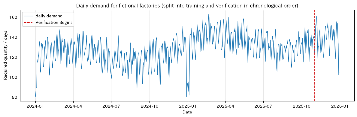
Daily data will be generated for two years starting from January 2024. Demand experiences gradual growth, weekday cycles, annual cycles, self-regressive fluctuations, and the impact of year-end and New Year holidays. Orders outpace demand, and production lags behind demand. Observation noise is added to the equipment temperature sensor.

In practice, defining deficiencies, closing times, units, returns, express orders, and stop dates are defined, using only explanatory variables that are actually available at the time of prediction.

dates = pd.date_range("2024-01-01", periods=730, freq="D")
n = len(dates)
t = np.arange(n)
weekday = dates.dayofweek.to_numpy()

trend = 118 + 0.035 * t
weekly = np.array([-4, 1, 4, 7, 5, -10, -14])[weekday]
annual = 9 * np.sin(2 * np.pi * t / 365.25) + 4 * np.cos(2 * np.pi * t / 365.25)
shutdown = np.asarray(((dates.month == 1) & (dates.day <= 4)) | ((dates.month == 12) & (dates.day >= 29)))

shock = np.zeros(n)
innovation = rng.normal(0, 5.0, n)
for i in range(2, n):
    shock[i] = 0.58 * shock[i - 1] - 0.18 * shock[i - 2] + innovation[i] + 0.25 * innovation[i - 1]

demand = trend + weekly + annual + shock - 38 * shutdown
orders = np.roll(demand, -2) + rng.normal(5, 6, n)
orders[-2:] = demand[-2:] + rng.normal(5, 6, 2)
production = 0.62 * np.roll(demand, 1) + 0.38 * demand + rng.normal(2, 4, n)
production[0] = demand[0] + rng.normal(2, 4)

true_temp = 61 + 0.012 * t + 1.8 * np.sin(2 * np.pi * t / 30)
sensor_temp = true_temp + rng.normal(0, 2.2, n)

df = pd.DataFrame({
    "Required quantity": demand.round(1),
    "Number of orders received": orders.round(1),
    "Production Quantity": production.round(1),
    "True Facility Temperature": true_temp,
    "sensor temperature": sensor_temp,
    "Closed day": shutdown.astype(int),
}, index=dates)

test_days = 60
train = df.iloc[:-test_days].copy()
test = df.iloc[-test_days:].copy()

display(df.head())
print(f"Period: {df.index.min().date()}〜{df.index.max().date()} / training: {len(train)}days / verification: {len(test)}days")

fig, ax = plt.subplots(figsize=(12, 4))
ax.plot(df.index, df["Required quantity"], lw=1, label="daily demand")
ax.axvline(test.index[0], color="tab:red", ls="--", label="Verification Begins")
ax.set_title("Daily demand for fictional factories (split into training and verification in chronological order)")
ax.set_xlabel("Date")
ax.set_ylabel("Required quantity / days")
ax.grid(alpha=0.3)
ax.legend()
plt.tight_layout()
plt.show()

	Required quantity	Number of orders received	Production Quantity	True Facility Temperature	sensor temperature	Closed day
2024-01-01	80.00	91.60	83.30	61.00	61.93	1
2024-01-02	85.20	93.20	80.40	61.39	62.61	1
2024-01-03	90.00	128.50	91.60	61.76	60.63	1
2024-01-04	89.50	127.10	100.10	62.09	61.13	1
2024-01-05	118.30	121.10	99.70	62.39	65.17	0

Period: 2024-01-01 – 2025-12-30 / Training: 670 days / Verification: 60 days

No.081: ACF — Checking the Temporal Memory of Demand

Meaning in Practice

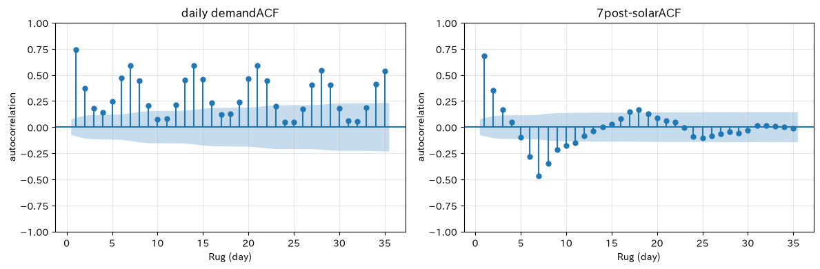
The Autocorrelation Function (ACF) measures how similar demand is to demand $k$ days ago. If correlations remain on lug 7, 14, and 21 days, it suggests day-of-the-week correlation; if it decays gently, it doubts trends or AR structures. Whether a correlation remains within the order lead time is a key factor in determining whether short-term forecasts can be used for inventory replenishment.

Approach to Analysis and Modeling

The sample autocorrelation for lag $k$ is generally

$r_k=\frac{\sum_{t=k+1}^{T}(y_t-\bar y)(y_{t-k}-\bar y)}{\sum_{t=1}^{T}(y_t-\bar y)^2}$

That’s right. However, ACF for trendy or seasonal series appears to be higher. We compare the original series with previous year’s and seasonal differences, and also check the structure after normalization.

Check with Python

acf_lags = [1, 2, 7, 14, 21, 28]
acf_table = pd.DataFrame({
    "Rug (day)": acf_lags,
    "Original SeriesACF": [train["Required quantity"].autocorr(lag=k) for k in acf_lags],
    "7daily differenceACF": [train["Required quantity"].diff(7).dropna().autocorr(lag=k) for k in acf_lags],
})
display(acf_table)

fig, axes = plt.subplots(1, 2, figsize=(12, 4))
plot_acf(train["Required quantity"], lags=35, ax=axes[0], zero=False)
axes[0].set_title("daily demandACF")
axes[0].set_xlabel("Rug (day)")
axes[0].set_ylabel("autocorrelation")
axes[0].grid(alpha=0.3)
plot_acf(train["Required quantity"].diff(7).dropna(), lags=35, ax=axes[1], zero=False)
axes[1].set_title("7post-solarACF")
axes[1].set_xlabel("Rug (day)")
axes[1].set_ylabel("autocorrelation")
axes[1].grid(alpha=0.3)
plt.tight_layout()
plt.show()

	Rug (day)	Original SeriesACF	7daily differenceACF
0	1	0.75	0.69
1	2	0.38	0.36
2	7	0.61	-0.49
3	14	0.61	-0.00
4	21	0.62	0.06
5	28	0.58	-0.05

Reading the results

In the original series, short-term correlations and 7-day cycles are visible, and there is some basis for simple forecasts that keep the level at the same level as yesterday. On the other hand, after a 7-day difference, many correlations weaken, and it becomes clear that part of the original’s high correlation comes from the timing of the week and trend. The order is not determined by ACF alone; instead, the residual ACF and the future period error are also checked.

No.082: PACF — Narrowing down the directly affected rugs

Meaning in Practice

PACF (Partial Autocorrelation) examines the direct relationship a lag has to demand after controlling for the impact of the days in between. If Lag 1 is strong, you can include information from the previous day; if Lag 7 remains, you can include information from the same day in the production plan.

Approach to Analysis and Modeling

The PACF of lag $k$ corresponds to the coefficient of $y_{t-k}$ when $y_t$ is regressed at $y_{t-1},\ldots,y_{t-k}$. In AR ($p$), PACF theoretically ends after $p$, so it can be used to select candidates for AR levels. However, if seasonality or irregularity remains, it cannot be read simply.

Check with Python

stationary_demand = train["Required quantity"].diff(7).dropna()
fig, ax = plt.subplots(figsize=(10, 4))
plot_pacf(stationary_demand, lags=28, method="ywm", ax=ax, zero=False)
ax.set_title("7Demand divided by the difference of dayPACF")
ax.set_xlabel("Rug (day)")
ax.set_ylabel("partial autocorrelation")
ax.grid(alpha=0.3)
plt.tight_layout()
plt.show()

from statsmodels.tsa.stattools import pacf
pacf_values = pacf(stationary_demand, nlags=14, method="ywm")
display(pd.DataFrame({"Rug (day)": np.arange(1, 15), "PACF": pacf_values[1:]}).sort_values("PACF", key=abs, ascending=False).head(7))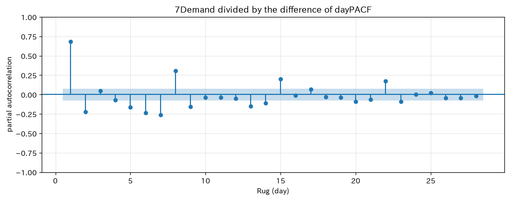

	Rug (day)	PACF
0	1	0.69
7	8	0.31
6	7	-0.26
5	6	-0.23
1	2	-0.23
4	5	-0.16
8	9	-0.15

Reading the results

Lags with strong partial autocorrelation are candidates for AR models, but “statistically significant” and “production plan-important” are not the same. We narrow down the candidate order to a small number and compare it with information quantification criteria such as AIC and time series verification. Excessive lag increases difficulty, making it difficult to explain and slowing down on structural changes.

No.083: AR Model — Forecasting Short-Term Demand from Past Demand

Meaning in Practice

The autoregressive (AR) model predicts the next demand based on recent demand performance. Ideal for short procurement lead times and daily personnel fine-tuning. On the other hand, unprecedented changes such as price revisions or new customer hiring cannot be predicted on your own.

Approach to Analysis and Modeling

AR ($p$)

$y_t=c+\phi_1y_{t-1}+\cdots+\phi_py_{t-p}+\varepsilon_t$

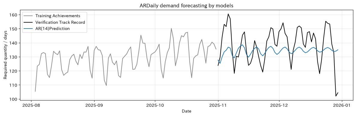
This is how it is expressed. Here, we use Lug 14 to include the weekly cycle. The validation period is fixed at the last 60 days, and RMSE and MAE are calculated without mixing future values into training.

Check with Python

ar_fit = AutoReg(train["Required quantity"], lags=14, trend="ct", old_names=False).fit()
ar_pred = ar_fit.predict(start=len(train), end=len(df) - 1, dynamic=False)
ar_pred.index = test.index

ar_metrics = pd.DataFrame({
    "Model": ["AR(14)"],
    "RMSE": [root_mean_squared_error(test["Required quantity"], ar_pred)],
    "MAE": [mean_absolute_error(test["Required quantity"], ar_pred)],
    "AIC": [ar_fit.aic],
})
display(ar_metrics)

fig, ax = plt.subplots(figsize=(12, 4))
ax.plot(train.index[-90:], train["Required quantity"].iloc[-90:], label="Training Achievements", color="0.55")
ax.plot(test.index, test["Required quantity"], label="Verification Track Record", color="black")
ax.plot(test.index, ar_pred, label="AR(14)Prediction", color="tab:blue")
ax.set_title("ARDaily demand forecasting by models")
ax.set_xlabel("Date")
ax.set_ylabel("Required quantity / days")
ax.grid(alpha=0.3)
ax.legend()
plt.tight_layout()
plt.show()

	Model	RMSE	MAE	AIC
0	AR(14)	12.14	9.96	4370.51

Reading the results

AR models track levels and short-term waves, but the longer the forecast, the easier it is to converge on the same recursive structure. MAE is the average required adjustment number, and RMSE is read as a strong penalty for major deviations. If there are heavy losses due to overcapacity or out-of-stock, do not decide on hiring based solely on symmetrical error indicators.

No.084: MA Model — Expressing the Aftermath of Temporary Shocks

Meaning in Practice

The Moving Average (MA) model represents a structure where past forecast errors remain in the present. It is suitable for processes where temporary shocks such as express orders, short stoppages, or early delivery can be resolved within a few days. Here, MA is different from smoothing using a simple moving average.

Approach to Analysis and Modeling

MA ($q$) is

$y_t=\mu+\varepsilon_t+\theta_1\varepsilon_{t-1}+\cdots+\theta_q\varepsilon_{t-q}$

That’s right. This time, we use MA(2) combined with trend elements to represent the unexplained shocks over the past two days. Since errors cannot be directly observed, they are estimated using the most likelihood method.

Check with Python

ma_fit = ARIMA(train["Required quantity"], order=(0, 0, 2), trend="ct").fit()
ma_forecast = ma_fit.get_forecast(steps=len(test))
ma_pred = pd.Series(ma_forecast.predicted_mean.to_numpy(), index=test.index)
ma_ci = ma_forecast.conf_int(alpha=0.05)

display(pd.DataFrame({
    "Model": ["MA(2)+trend"],
    "RMSE": [root_mean_squared_error(test["Required quantity"], ma_pred)],
    "MAE": [mean_absolute_error(test["Required quantity"], ma_pred)],
    "AIC": [ma_fit.aic],
}))

fig, ax = plt.subplots(figsize=(12, 4))
ax.plot(test.index, test["Required quantity"], label="Verification Track Record", color="black")
ax.plot(test.index, ma_pred, label="MA(2)Prediction", color="tab:orange")
ax.fill_between(test.index, ma_ci.iloc[:, 0], ma_ci.iloc[:, 1], color="tab:orange", alpha=0.2, label="95%Predicted Section")
ax.set_title("MADemand forecasting and forecast sections by model")
ax.set_xlabel("Date")
ax.set_ylabel("Required quantity / days")
ax.grid(alpha=0.3)
ax.legend()
plt.tight_layout()
plt.show()

	Model	RMSE	MAE	AIC
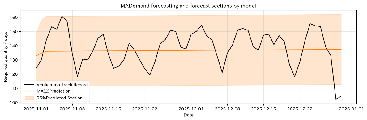
0	MA(2)+trend	12.64	10.32	4712.80

Reading the results

MA(2) can represent short-term shocks, but since it lacks explicit weekly days, it cannot fully capture weekly ups and downs. The forecast interval is not a confidence interval for average demand, but a range that allows for individual future observations. In safety stock, the upper quantile is important, but the error distribution and cumulative demand during lead time are considered separately.

No.085: ARIMA — Modeling Change by Difference

Meaning in Practice

When demand levels increase or decrease, models assuming constant averages are pulled back to old levels. ARIMA handles level changes based on differences and can be used for baseline forecasting during startup periods or during moderate market growth.

Approach to Analysis and Modeling

ARIMA ($p,d,q$) assigns ARMA ($p,q$) to the series of $d$ differences. The first floor difference is $\Delta y_t=y_t-y_{t-1}$. Here, ARIMA(2,1,2) will be used. To amplify noise if the difference order is too high, graphs, root of unit tests, residuals, and future precision are used together.

Check with Python

arima_fit = ARIMA(train["Required quantity"], order=(2, 1, 2), trend="t").fit()
arima_fc = arima_fit.get_forecast(steps=len(test))
arima_pred = pd.Series(arima_fc.predicted_mean.to_numpy(), index=test.index)
arima_ci = arima_fc.conf_int()

display(pd.DataFrame({
    "Model": ["ARIMA(2,1,2)"],
    "RMSE": [root_mean_squared_error(test["Required quantity"], arima_pred)],
    "MAE": [mean_absolute_error(test["Required quantity"], arima_pred)],
    "AIC": [arima_fit.aic],
}))

fig, axes = plt.subplots(1, 2, figsize=(13, 4))
axes[0].plot(train.index[-120:], train["Required quantity"].iloc[-120:])
axes[0].set_title("Demand Level (before diff)")
axes[0].set_xlabel("Date")
axes[0].set_ylabel("Required quantity / days")
axes[0].grid(alpha=0.3)
axes[1].plot(test.index, test["Required quantity"], label="Achievements", color="black")
axes[1].plot(test.index, arima_pred, label="ARIMAPrediction", color="tab:green")
axes[1].fill_between(test.index, arima_ci.iloc[:, 0], arima_ci.iloc[:, 1], color="tab:green", alpha=0.2)
axes[1].set_title("ARIMAPrediction")
axes[1].set_xlabel("Date")
axes[1].set_ylabel("Required quantity / days")
axes[1].grid(alpha=0.3)
axes[1].legend()
plt.tight_layout()
plt.show()

	Model	RMSE	MAE	AIC
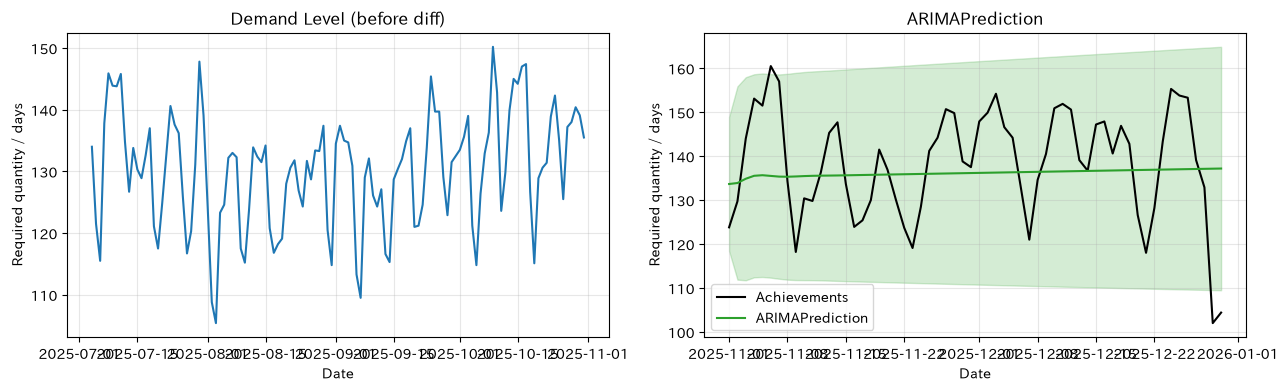
0	ARIMA(2,1,2)	12.71	10.39	4658.08

Reading the results

ARIMA follows local level changes but does not specify weekly patterns. AIC is used for relative comparisons between candidates applying the same data and is treated separately from operational losses in different verification intervals. If the residual has a 7-day cycle left, the next SARIMA is a natural candidate.

No.086: SARIMA — Forecasting Production Volume Including Date of the Week

Meaning in Practice

In factories where order and shipping patterns differ by day of the week, ignoring seasonality results in stockouts on the same day every week. SARIMA adds seasonal differences and seasonal AR/MA to the standard ARIMA, expressing repetition of regular cycles such as weekly and monthly.

Approach to Analysis and Modeling

SARIMA writes $(p,d,q)\times(P,D,Q)_s$. $s=7$ is the weekly cycle of daily data. This time, we will $(1,1,1)\times(1,0,1)_7$ and keep the complexity down. If holidays are moving or equipment stoppages are irregular, add exogenous variables.

Check with Python

sarima_fit = SARIMAX(
    train["Required quantity"],
    order=(1, 1, 1),
    seasonal_order=(1, 0, 1, 7),
    trend="t",
    enforce_stationarity=False,
    enforce_invertibility=False,
).fit(disp=False)
sarima_fc = sarima_fit.get_forecast(steps=len(test))
sarima_pred = pd.Series(sarima_fc.predicted_mean.to_numpy(), index=test.index)
sarima_ci = sarima_fc.conf_int()

model_metrics = pd.DataFrame({
    "Model": ["AR(14)", "MA(2)+trend", "ARIMA(2,1,2)", "SARIMA-weekly"],
    "RMSE": [
        root_mean_squared_error(test["Required quantity"], ar_pred),
        root_mean_squared_error(test["Required quantity"], ma_pred),
        root_mean_squared_error(test["Required quantity"], arima_pred),
        root_mean_squared_error(test["Required quantity"], sarima_pred),
    ],
    "MAE": [
        mean_absolute_error(test["Required quantity"], ar_pred),
        mean_absolute_error(test["Required quantity"], ma_pred),
        mean_absolute_error(test["Required quantity"], arima_pred),
        mean_absolute_error(test["Required quantity"], sarima_pred),
    ],
}).sort_values("RMSE")
display(model_metrics)

fig, ax = plt.subplots(figsize=(12, 4))
ax.plot(test.index, test["Required quantity"], label="Verification Track Record", color="black", lw=1.5)
ax.plot(test.index, sarima_pred, label="SARIMAPrediction", color="tab:red")
ax.fill_between(test.index, sarima_ci.iloc[:, 0], sarima_ci.iloc[:, 1], color="tab:red", alpha=0.18, label="95%Predicted Section")
ax.set_title("Including weekly seasonalitySARIMADemand forecasting")
ax.set_xlabel("Date")
ax.set_ylabel("Required quantity / days")
ax.grid(alpha=0.3)
ax.legend()
plt.tight_layout()
plt.show()

	Model	RMSE	MAE
0	AR(14)	12.14	9.96
1	MA(2)+trend	12.64	10.32
2	ARIMA(2,1,2)	12.71	10.39
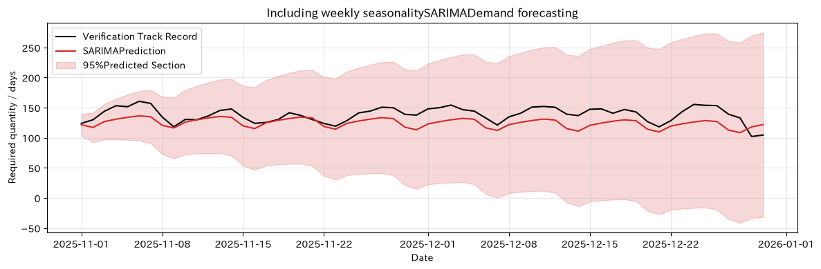
3	SARIMA-weekly	17.13	15.12

Reading the results

Despite clearly specifying the day of the week in this SARIMA case, RMSE and MAE performance worsened compared to simple AR. Including seasonal items does not guarantee improvement; the error factor is that the trend specifications and the year-end holiday at the end of the verification are not explained. Instead of rejecting results in a single round, we roll and verify the degree and holiday exogenous variables. On days when the forecasted section limit exceeds production capacity, rules for early production and outsourcing are linked.

No.087: VAR — Modeling the interactions of demand, orders, and production

Meaning in Practice

Instead of just demand alone, handling both leading orders and following production simultaneously allows you to grasp the time gap between supply and demand. VAR explains multiple series using their historical values, forming the foundation for creating common scenarios between sales and production management.

Approach to Analysis and Modeling

$K$ The variable VAR($p$) is

$\mathbf y_t=\mathbf c+A_1\mathbf y_{t-1}+\cdots+A_p\mathbf y_{t-p}+\boldsymbol\varepsilon_t$

That’s right. To avoid false regression at unsteady levels, we use first-order differences here. As the number of series and lags increases, parameters increase rapidly, prioritizing data volume and business interpretation.

Check with Python

var_cols = ["Required quantity", "Number of orders received", "Production Quantity"]
var_train_diff = train[var_cols].diff().dropna()
var_fit = VAR(var_train_diff).fit(maxlags=7, ic="aic")
horizon = 14
diff_fc = var_fit.forecast(var_train_diff.to_numpy()[-var_fit.k_ar:], steps=horizon)
var_levels = train[var_cols].iloc[-1].to_numpy() + np.cumsum(diff_fc, axis=0)
var_forecast = pd.DataFrame(var_levels, index=test.index[:horizon], columns=var_cols)

print(f"AICLag order selected by: {var_fit.k_ar}")
display(var_forecast.head())

fig, axes = plt.subplots(3, 1, figsize=(12, 8), sharex=True)
for ax, col in zip(axes, var_cols):
    ax.plot(test.index[:horizon], test[col].iloc[:horizon], label="Achievements", color="black")
    ax.plot(var_forecast.index, var_forecast[col], label="VARPrediction", color="tab:purple")
    ax.set_title(f"VARaccording to{col}of14Forecast for the day")
    ax.set_xlabel("Date")
    ax.set_ylabel("quantity / days")
    ax.grid(alpha=0.3)
    ax.legend()
plt.tight_layout()
plt.show()

Number of lags selected by AIC: 7

	Required quantity	Number of orders received	Production Quantity
2025-11-01	124.63	145.22	133.53
2025-11-02	129.16	147.47	129.57
2025-11-03	137.48	145.05	136.03
2025-11-04	139.19	146.75	141.50
2025-11-05	139.17	143.29	142.63

Reading the results

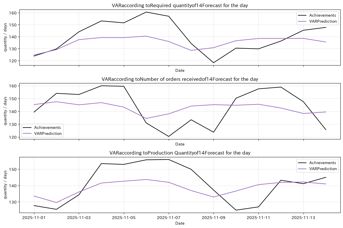
By forecasting all three lines on the same timeline, you can check whether production can keep pace with increased demand. However, the VAR coefficient is not a causal effect. Orders can anticipate future demand in terms of generational timing, and in production, the input confirmation time and data revision are audited. This structure is better suited for detecting short-term supply-demand gaps rather than long-term forecasting.

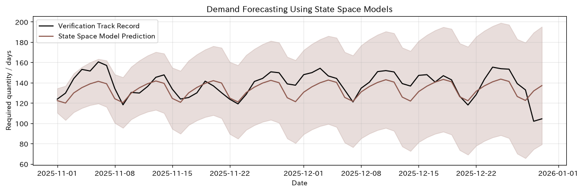
No.088: State Space Model — Estimating the Underlying Tone of Observations

Meaning in Practice

Daily demand includes noise, but production capacity and purchasing contracts should be decided according to the overall situation. The state-space model classifies unobservable demand levels, slopes, and seasonal components as states, flexibly responding to missing measurements and irregular changes.

Approach to Analysis and Modeling

The general form consists of observational equations and state equations.

$y_t=Z_t\alpha_t+\varepsilon_t,\qquad \alpha_{t+1}=T_t\alpha_t+\eta_t$

That’s right. $\alpha_t$ is the latent state, $\varepsilon_t$ is the observation error, and $\eta_t$ is the state change. Here, we estimate local linear trends and weekly seasonal components.

Check with Python

ucm = UnobservedComponents(
    train["Required quantity"],
    level="local linear trend",
    seasonal=7,
    autoregressive=2,
)
ucm_fit = ucm.fit(disp=False)
ucm_fc = ucm_fit.get_forecast(steps=len(test))
ucm_pred = pd.Series(ucm_fc.predicted_mean.to_numpy(), index=test.index)
ucm_ci = ucm_fc.conf_int()

display(pd.DataFrame({
    "Model": ["State space (local linear+weekly+AR2）"],
    "RMSE": [root_mean_squared_error(test["Required quantity"], ucm_pred)],
    "MAE": [mean_absolute_error(test["Required quantity"], ucm_pred)],
    "AIC": [ucm_fit.aic],
}))

fig, ax = plt.subplots(figsize=(12, 4))
ax.plot(test.index, test["Required quantity"], label="Verification Track Record", color="black")
ax.plot(test.index, ucm_pred, label="State Space Model Prediction", color="tab:brown")
ax.fill_between(test.index, ucm_ci.iloc[:, 0], ucm_ci.iloc[:, 1], color="tab:brown", alpha=0.2)
ax.set_title("Demand Forecasting Using State Space Models")
ax.set_xlabel("Date")
ax.set_ylabel("Required quantity / days")
ax.grid(alpha=0.3)
ax.legend()
plt.tight_layout()
plt.show()

	Model	RMSE	MAE	AIC
0	State space (local linear+weekly+AR2）	11.26	8.90	4364.45

Reading the results

In addition to prediction, state-space models express “how much the underlying tone will move” as state variance. If you allow too much change, it will overfit noise; if you don’t, it will not follow structural changes. The key point of implementation is to match model parts with business knowledge and monitor state variance, residuals, and coverage rates in predicted sections.

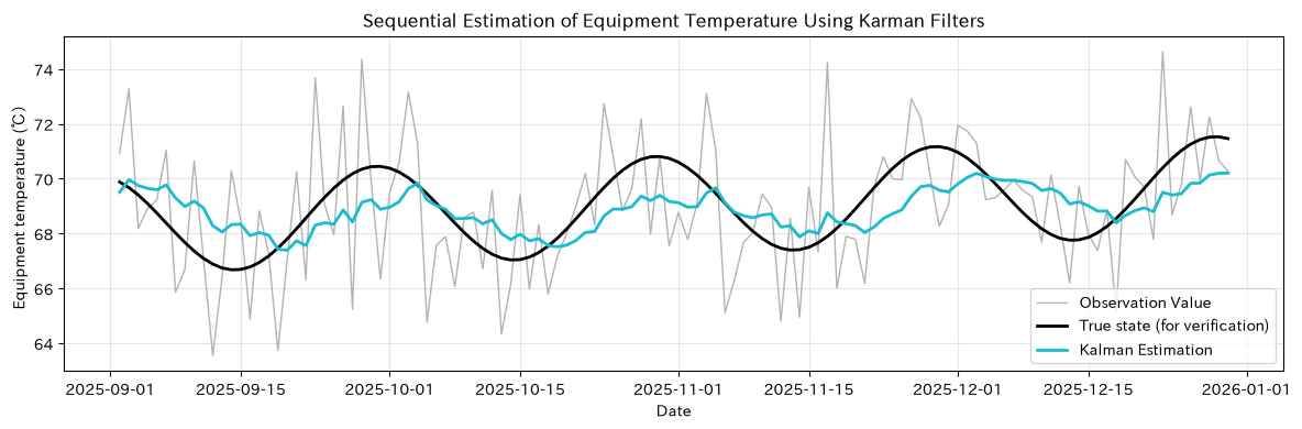
No.089: Karman Filter — Sequentially Estimating Equipment Status

Meaning in Practice

Temperature, vibration, and pressure sensors contain noise. Applying thresholds directly to observations increases false alarms. The Kalman filter updates state estimates whenever new measurements arrive, creating stable input for preventive maintenance and anomaly monitoring.

Approach to Analysis and Modeling

Forecasts and updates are repeated. In one-dimensional local-level models, predicted variance $P_{t|t-1}=P_{t-1|t-1}+Q$, Kalman gain,

$K_t=\frac{P_{t|t-1}}{P_{t|t-1}+R}$

Update value $\hat x_{t|t}=\hat x_{t|t-1}+K_t(y_t-\hat x_{t|t-1})$. $Q$ is the true state change, and $R$ is the dispersion of observed noise.

Check with Python

observations = df["sensor temperature"].to_numpy()
q, r = 0.08, 2.2**2
x_est, p = observations[0], 10.0
filtered, gains = [], []

for y in observations:
    x_pred = x_est
    p_pred = p + q
    k = p_pred / (p_pred + r)
    x_est = x_pred + k * (y - x_pred)
    p = (1 - k) * p_pred
    filtered.append(x_est)
    gains.append(k)

df["Calman Estimated Temperature"] = filtered
sensor_rmse = root_mean_squared_error(df["True Facility Temperature"], df["sensor temperature"])
kalman_rmse = root_mean_squared_error(df["True Facility Temperature"], df["Calman Estimated Temperature"])
display(pd.DataFrame({
    "series": ["Raw sensor", "Kalman Estimation"],
    "For the true stateRMSE": [sensor_rmse, kalman_rmse],
    "Most recent Karman Gains": [np.nan, gains[-1]],
}))

fig, ax = plt.subplots(figsize=(12, 4))
window = df.iloc[-120:]
ax.plot(window.index, window["sensor temperature"], color="0.7", lw=1, label="Observation Value")
ax.plot(window.index, window["True Facility Temperature"], color="black", lw=2, label="True state (for verification)")
ax.plot(window.index, window["Calman Estimated Temperature"], color="tab:cyan", lw=2, label="Kalman Estimation")
ax.set_title("Sequential Estimation of Equipment Temperature Using Karman Filters")
ax.set_xlabel("Date")
ax.set_ylabel("Equipment temperature (℃）")
ax.grid(alpha=0.3)
ax.legend()
plt.tight_layout()
plt.show()

	series	For the true stateRMSE	Most recent Karman Gains
0	Raw sensor	2.23	NaN
1	Kalman Estimation	1.17	0.12

Reading the results

The RMSE of the estimated series is lower than that of the raw sensor, which suppresses short-term noise. However, since it can delay sudden true changes, do not judge safe stops based solely on the smoothed values. $Q$ and $R$ adjust maintenance history, calibration tests, and pseudo-abnormalities, and assign roles to soft alerts for raw value hard thresholds and state estimation.

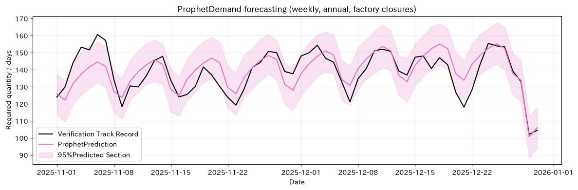
No.090: Prophet — Breaking Trends, Seasonality, and Holidays into Explainable Parts

Meaning in Practice

Prophet is a model that additively represents trends, weekly and annual seasonality, and holiday effects, making it easy to explain calendar factors. It is easy to share with sales and production management about “which days of the week the increase will increase” and “how much will decrease due to closure,” making it suitable as a benchmark model for regular relearning.

Approach to Analysis and Modeling

The basic form is

$y(t)=g(t)+s(t)+h(t)+\varepsilon_t$

$g(t)$ is the periodic trend, $s(t)$ is the seasonality of the Fourier series, and $h(t)$ is the holiday effect. Since increasing flexibility can easily lead to overfitting, changepoints, seasonality, and holiday windows are matched with business changes.

Check with Python

prophet_train = train.reset_index().rename(columns={"index": "ds", "Required quantity": "y"})[["ds", "y"]]
holiday_dates = df.index[df["Closed day"].eq(1)]
holidays = pd.DataFrame({"holiday": "factory closure", "ds": holiday_dates})

prophet_model = Prophet(
    holidays=holidays,
    weekly_seasonality=True,
    yearly_seasonality=True,
    daily_seasonality=False,
    interval_width=0.95,
    changepoint_prior_scale=0.05,
)
prophet_model.fit(prophet_train)
future = pd.DataFrame({"ds": test.index})
prophet_fc = prophet_model.predict(future).set_index("ds")

display(pd.DataFrame({
    "Model": ["Prophet"],
    "RMSE": [root_mean_squared_error(test["Required quantity"], prophet_fc["yhat"])],
    "MAE": [mean_absolute_error(test["Required quantity"], prophet_fc["yhat"])],
    "Interval Ratio": [((test["Required quantity"] >= prophet_fc["yhat_lower"]) & (test["Required quantity"] <= prophet_fc["yhat_upper"])).mean()],
}))

fig, ax = plt.subplots(figsize=(12, 4))
ax.plot(test.index, test["Required quantity"], color="black", label="Verification Track Record")
ax.plot(prophet_fc.index, prophet_fc["yhat"], color="tab:pink", label="ProphetPrediction")
ax.fill_between(prophet_fc.index, prophet_fc["yhat_lower"], prophet_fc["yhat_upper"], color="tab:pink", alpha=0.2, label="95%Predicted Section")
ax.set_title("ProphetDemand forecasting (weekly, annual, factory closures)")
ax.set_xlabel("Date")
ax.set_ylabel("Required quantity / days")
ax.grid(alpha=0.3)
ax.legend()
plt.tight_layout()
plt.show()

	Model	RMSE	MAE	Interval Ratio
0	Prophet	7.55	6.05	0.88

Reading the results

Prophet expresses demand decline due to closures and seasonality separately, and can also check the coverage rate of the forecast area. If the proportion within the interval deviates significantly from the nominal 95%, uncertainty is underestimated or overestimated. Even with convenient automation, it is the user’s responsibility to register future holidays, change order systems, and manage without mixing unknown information at the time of forecasting.

Practical Implications Seen Through Target Exercise

1. Start with a diagnosis: After reviewing the time structure in ACF and PACF, we create degree candidates and do not decide on model names first.
2. Evaluate in the future: Use time-series holdout and rolling verification to prevent leaks caused by random splitting.
3. Translating point predictions into business decisions: Match forecast interval limits and capacity, quantiles and safety stock, forecast errors, and out-of-stock losses.
4. Distinguishing between univariate and multivariate measures: Advance information such as orders is useful, but always confirm that it is finalized at the time of forecasting.
5. Distinguishing State Estimation from Safety Control: Kalman filters are effective for noise reduction but carry the risk of delaying sudden changes.
6. Not fixing on a single winner: Continuously compare candidates including simple baseline models according to seasonality, structural changes, and forecast periods.

What is necessary for practical implementation

• Definition of decision-making: Clearly state forecasting targets, granularity, lead time, cutoff time, update frequency, and users
• Data Contracts: Record missing items, cancellations, returns, business closures, express orders, unit changes, and master revisions
• Verification Design: Rolling validation evaluates multiple seasons and measures not only RMSE but also out-of-stock, inventory, and overtime costs.
• Operation of Uncertainty: Establish rules for early production, outsourcing, additional orders, and administrator approval for each forecast section
• surveillance: Record prediction errors, interval coverage rates, residual autocorrelation, input distributions, missed test rates, and calculation errors.
• Change management: Reflecting structural changes such as facility expansion, price revisions, large customers, and holidays in the model, and preserving a relearning history
• Boundary of Responsibility: Clarify the scope proposed by the model and approved by the site, along with hard safety and quality constraints.

Conclusion

From No.081 to No.090, diagnostics using ACF and PACF were implemented, covering everything from AR, MA, ARIMA, SARIMA, VAR, state space models, Karman filters, to Prophet using the same hypothetical factory data.

The value of time series analysis is not in choosing the most complex model. It is about visualizing time structures and uncertainties, connecting them to inventory, capacity, and maintenance judgment rules, and creating a system that can improve after errors. First, prepare simple baseline forecasts and time series validations, then add complexity that can be explained in business terms.

Consultations for Corporations

At Sukari Kobo, we support manufacturing industry from demand forecasting, production and inventory planning, equipment condition estimation, time-series data platforms, Python training, and PoC to operational implementation. From stages such as “There is forecasting but it does not lead to ordering decisions,” “I want to design model accuracy monitoring,” or “There are issues with the timing, loss, or master of field data,” we organize both business requirements and data.

📩 Contact Us: surikobo.co.jp/contact
Please feel free to consult us first.