Eigenvalue Analysis to Detect ‘Amplification and Convergence’ of Process Variations — 100 Exercises on Linear Algebra in Manufacturing No.041–No.050

On the production line, dimensional deviations from previous processes, equipment vibration, temperature deviations, and other factors influence each other and are transmitted to the quality status the next day. In this article, we use a fictional line consisting of three processes as a subject, and examine Eigenvalues, eigenvectors, diagonalization, duplication, polynomials, Jordan canon, spectral decomposition, positive definite matrices in a way that leads to equipment adjustment and quality judgment.

The key point is not to calculate formulas, but to be able to explain (1) which modes of variation remain, (2) whether the effects converge in the long term, and (3) whether the evaluation indicators can be used safely. The published data is fictional generated in Python and does not depend on external data.

[!NOTE] This material is a notebook previously used by Surikoubo (or personally by the representative, Kazuyama), and has been reconstructed, edited, and published with the company’s permission.
All data listed is fictional and has no relation whatsoever to real companies, factories, or figures.

Introduction: Practical Challenges in Manufacturing Covered in This Article

Suppose a precision parts line records the standardization deviations of machining, heat treatment, and inspection on a daily basis. If we $\mathbf{x}_t$ the quality deviation vector and let the matrix representing propagation between processes be $A$, the simplified state update is

$\mathbf{x}_{t+1}=A\mathbf{x}_t+\boldsymbol{\varepsilon}_t$

That’s right. $\boldsymbol{\varepsilon}_t$ is a small disturbance that joins the day. What you want to know is not just individual coefficients. It is necessary to determine how many times the deviation remains, which process combinations it presents, and whether it converges after adjustment.

Common situations on site

• Even if the control charts for each process are normal, gradual fluctuations across processes may still remain.
• As a result of narrowing the adjustment target to a single process, deviations from other processes increase.
• Simulations are possible, but long-term stability cannot be explained.
• Optimization is being carried out without verifying whether the weight matrix of the quality score is valid.

Why is this issue so difficult to judge?

Each element of matrix $A$ is a local influence. On the other hand, what the site needs “what will happen in a certain number of days” is determined by $A^k$ and cannot be understood by simply observing the elements. The eigenvalue is the multiplier of the variation mode, while the eigenvector gives the process composition. However, for duplicate eigenvalues or non-diagonalizable matrices, simple interpretations fail, so it is necessary to check the degree of duplication and even the minimal polynomial.

Overview of Exercise covered this time

No.	Theme	Practical Questions
041	eigenvalue	Do fluctuations amplify or attenuate?
042	eigenvector	Which process combinations dominate?
043	diagonalization	Can you simply calculate transmission many days ahead?
044	geometric repetition	How many independent directions of change are there?
045	algebraic repetition	How many times does the same multiplier appear on the equation?
046	characteristic polynomial	Can eigenvalues be checked from definition expressions?
047	minimal polynomial	What is the smallest relation to eliminate a matrix?
048	Jordan Standard Form	How to interpret temporary amplification when diagonalization is impossible
049	spectral decomposition	Can fluctuations be broken down by orthogonal mode?
050	positive definite matrix	Whether the quality score is always a non-negative and unique evaluation

Preparing the Python environment

Perform matrix calculations with NumPy, tables with pandas, and visualization with Matplotlib. To ensure reproducibility, the random number generator seed is fixed. The displayed rounding and calculation accuracy are separated, and judgments are made using the values before rounding.

import sys
import numpy as np
import pandas as pd
import matplotlib
import matplotlib.pyplot as plt
from IPython.display import display

np.set_printoptions(precision=4, suppress=True)
rng = np.random.default_rng(20260712)
print(f"Python {sys.version.split()[0]} / NumPy {np.__version__} / pandas {pd.__version__} / Matplotlib {matplotlib.__version__}")

Python 3.13.1 / NumPy 2.5.1 / pandas 3.0.3 / Matplotlib 3.11.0

Creation of Fictional Data

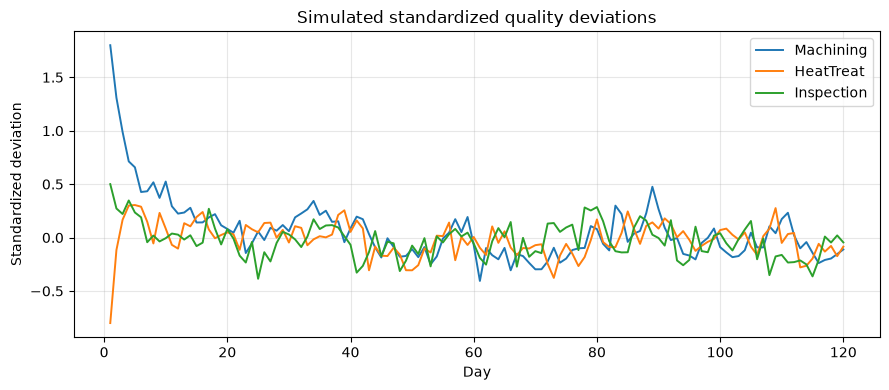
Generates 120 days’ worth of standardization deviations for the three processes. The propagation matrix $A$ is a symmetric matrix, and in practice, we set the structure where ‘the adjacent process has a stronger impact.’ Since the maximum eigenvalue is less than 1, if there is no disturbance, the deviation will decrease over the long term. Here, I will not jump to this conclusion and will verify it with each exercise.

processes = ["Machining", "HeatTreat", "Inspection"]
A = np.array([[0.72, 0.12, 0.04],
              [0.12, 0.58, 0.10],
              [0.04, 0.10, 0.46]])
n_days = 120
states = np.zeros((n_days, 3))
states[0] = [1.8, -0.8, 0.5]
for t in range(n_days - 1):
    states[t + 1] = A @ states[t] + rng.normal(0, 0.12, 3)
quality_df = pd.DataFrame(states, columns=processes).assign(Day=np.arange(1, n_days + 1))
display(pd.DataFrame(A, index=processes, columns=processes).round(2))
display(quality_df.head().round(3))

fig, ax = plt.subplots(figsize=(9, 4))
for col in processes:
    ax.plot(quality_df["Day"], quality_df[col], label=col, linewidth=1.4)
ax.set_title("Simulated standardized quality deviations")
ax.set_xlabel("Day"); ax.set_ylabel("Standardized deviation")
ax.grid(True, alpha=0.3); ax.legend(); fig.tight_layout(); plt.show()

	Machining	HeatTreat	Inspection
Machining	0.72	0.12	0.04
HeatTreat	0.12	0.58	0.10
Inspection	0.04	0.10	0.46

	Machining	HeatTreat	Inspection	Day
0	1.800	-0.800	0.500	1
1	1.309	-0.116	0.272	2
2	0.988	0.167	0.221	3
3	0.713	0.299	0.347	4
4	0.657	0.304	0.234	5

No.041: What is an eigenvalue?

Meaning in Practice

Eigenvalues represent how many times a specific fluctuation mode multiplies over a single period when the effects are repeated between processes. If there is an eigenvalue with an absolute value greater than 1, that mode amplifies even without disturbances, so the adjustment rules need to be reviewed.

Approach to Analysis and Modeling

For a nonzero vector $\mathbf{v}$, when multiplying by a matrix does not change orientation and only the multiplier becomes $\lambda$, $\lambda$ is called an eigenvalue. For the primary stability assessment, the spectral radius $\rho(A)=\max_i|\lambda_i|$ is used.

$A\mathbf{v}=\lambda\mathbf{v},\qquad \rho(A)<1\Rightarrow A^k\mathbf{x}_0\to\mathbf{0}$

Check with Python

eigvals = np.linalg.eigvalsh(A)
eigenvalue_table = pd.DataFrame({"Eigenvalue": eigvals[::-1], "Magnitude": np.abs(eigvals[::-1])})
display(eigenvalue_table.round(4))
rho = np.max(np.abs(eigvals))
print(f"Spectral radius = {rho:.4f}; asymptotically stable = {rho < 1}")

fig, ax = plt.subplots(figsize=(7, 3.5))
ax.bar(range(1, 4), eigvals[::-1], color="#2878B5")
ax.axhline(1, color="crimson", linestyle="--", label="stability boundary")
ax.set_title("Eigenvalues of the process propagation matrix")
ax.set_xlabel("Mode rank"); ax.set_ylabel("Eigenvalue")
ax.set_xticks([1, 2, 3]); ax.grid(True, axis="y", alpha=0.3); ax.legend(); fig.tight_layout(); plt.show()

	Eigenvalue	Magnitude
0	0.8102	0.8102
1	0.5487	0.5487
2	0.4010	0.4010

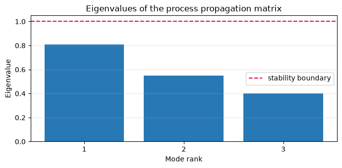
Spectral radius = 0.8102; asymptotically stable = True

Reading the results

The maximum eigenvalue (spectral radius) is about 0.82, less than 1. Therefore, if only the propagation is set, all modes will be attenuated. However, the 0.82 mode has the slowest attenuation and tends to persist when daily disturbances overlap, making it a top monitoring target.

No.042: What is an eigenvector?

Meaning in Practice

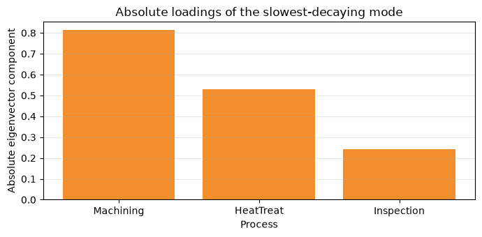
A eigenvector is a combination of processes that move together at the same magnification. By looking at the vector corresponding to the maximum eigenvalue, you can identify which process the long-lasting quality deviation includes simultaneously.

Approach to Analysis and Modeling

The entire sign of an eigenvector represents the same direction even when inverted. Therefore, rather than the positive or negative values themselves, we read the absolute values of components and the relative codes between processes. In symmetric matrices, eigenvectors can be selected as vectors of length 1 that are perpendicular to each other.

$A V=V\Lambda,\qquad V^\mathsf{T}V=I$

Check with Python

eigvals, eigvecs = np.linalg.eigh(A)
order = np.argsort(eigvals)[::-1]
eigvals, eigvecs = eigvals[order], eigvecs[:, order]
# For readability, the components with the highest absolute values in each vector are positively aligned.
eigvecs *= np.sign(eigvecs[np.argmax(np.abs(eigvecs), axis=0), range(3)])
loading_df = pd.DataFrame(eigvecs, index=processes, columns=[f"Mode {i+1}" for i in range(3)])
display(loading_df.round(3))

fig, ax = plt.subplots(figsize=(7, 3.5))
ax.bar(processes, np.abs(eigvecs[:, 0]), color="#F28E2B")
ax.set_title("Absolute loadings of the slowest-decaying mode")
ax.set_xlabel("Process"); ax.set_ylabel("Absolute eigenvector component")
ax.grid(True, axis="y", alpha=0.3); fig.tight_layout(); plt.show()

	Mode 1	Mode 2	Mode 3
Machining	0.812	-0.575	0.095
HeatTreat	0.529	0.660	-0.534
Inspection	0.244	0.484	0.840

Reading the results

Mode 1, which has the slowest attenuation, is heavily influenced by processing and heat treatment, and inspection is included in the same direction. Rather than treating it as a single-process abnormality, it is more appropriate to conduct a cross-disciplinary cause investigation that checks machining conditions and thermal history together. The eigenvector is not the causal relationship itself, but a hypothesis that indicates the priority of the investigation.

No.043: Diagonalization

Meaning in Practice

With diagonalization, multi-day impact $A^k$ can be calculated as independent multipliers for each mode $\lambda_i^k$. This improves the explanatory and computational efficiency of long-term simulations.

Approach to Analysis and Modeling

If a matrix $V$ with independent eigenvectors is regular, it can be decomposed to $A=V\Lambda V^{-1}$. In symmetrical $A$, it is $V^{-1}=V^\mathsf{T}$. Move the initial deviation to the mode coordinates, multiply by the magnification, and return to the process coordinates.

$A^k=V\Lambda^kV^{-1},\qquad \mathbf{x}_k=V\Lambda^kV^{-1}\mathbf{x}_0$

Check with Python

k = 12
Lambda = np.diag(eigvals)
A_k_direct = np.linalg.matrix_power(A, k)
A_k_diag = eigvecs @ np.linalg.matrix_power(Lambda, k) @ eigvecs.T
x0 = states[0]
comparison = pd.DataFrame({
    "Direct": A_k_direct @ x0,
    "Diagonalized": A_k_diag @ x0,
    "Absolute error": np.abs((A_k_direct - A_k_diag) @ x0)
}, index=processes)
display(comparison.round(10))
print(f"matrix reconstruction error = {np.linalg.norm(A - eigvecs @ Lambda @ eigvecs.T):.2e}")

	Direct	Diagonalized	Absolute error
Machining	0.076042	0.076042	0.0
HeatTreat	0.048527	0.048527	0.0
Inspection	0.022203	0.022203	0.0

matrix reconstruction error = 4.75e-16

Reading the results

After 12 days, the deviation matches the direct calculation and diagonalization, with errors of about a floating-point rounding. Since the maximum eigenvalue to the 12th power decreases, the deviation without disturbances is greatly attenuated. In practice, it is reasonable to assume that $A$ remains constant throughout the period, and we check every equipment modification or product change.

No.044: Repetition in Geometry

Meaning in Practice

How many independent eigenvectors for the same eigenvalue means the number of independent variation patterns with the same attenuation rate. If it is insufficient, it cannot be diagonalized, and polynomial terms are mixed into the predicted behavior.

Approach to Analysis and Modeling

The geometric redundancy of eigenvalue $\lambda$ is the dimension of the zero space of $A-\lambda I$. Numerical calculations set allowable errors for the singular values and determine the rank. Here, for explanation, we use a diagonal matrix with a overlapping eigenvalue of 2.

$g_\lambda=\dim\ker(A-\lambda I)=n-\operatorname{rank}(A-\lambda I)$

Check with Python

B = np.diag([2.0, 2.0, 0.5])
lam = 2.0
rank = np.linalg.matrix_rank(B - lam * np.eye(3))
geom_mult = B.shape[0] - rank
print("Example matrix B:\n", B)
print(f"rank(B - {lam}I) = {rank}")
print(f"Geometric multiplicity of lambda={lam} = {geom_mult}")
print("Independent directions: e1 and e2")

Example matrix B:
 [[2.  0.  0. ]
 [0.  2.  0. ]
 [0.  0.  0.5]]
rank(B - 2.0I) = 1
Geometric multiplicity of lambda=2.0 = 2
Independent directions: e1 and e2

Reading the results

The eigenvalue 2 has two independent directions, allowing distinguishing two independent phenomena with the same amplification rate. For example, it can handle situations where two independent units have the same attenuation rate. In numerical data, do not label “nearly identical eigenvalues” as duplicates; instead, clearly state measurement errors and tolerances.

No.045: The Repetition of Algebra

Meaning in Practice

Algebraic redundancy is how many times the same eigenvalue appears as the root of a characteristic polynomial. By comparing it with geometric duplication, you can determine whether a matrix can be diagonalized.

Approach to Analysis and Modeling

$1\le g_\lambda\le a_\lambda$ always holds. If the geometric and algebraic overlaps match all eigenvalues and their sum reaches the dimension, diagonalization is possible. Here, we look at an example where there is only one independent eigenvector with a degree of duplication of 2.

$a_\lambda:\ \det(\mu I-A)\text{ The root of }\lambda\text{ Number of duplicates}$

Check with Python

C = np.array([[0.8, 1.0, 0.0],
              [0.0, 0.8, 0.0],
              [0.0, 0.0, 0.3]])
roots = np.roots(np.poly(C))
alg_mult = int(np.sum(np.isclose(roots, 0.8)))
geom_mult = C.shape[0] - np.linalg.matrix_rank(C - 0.8 * np.eye(3))
display(pd.DataFrame({"Measure": ["Algebraic multiplicity", "Geometric multiplicity"],
                      "Value": [alg_mult, geom_mult]}))
print("Eigenvalues:", roots)
print("Diagonalizable:", alg_mult == geom_mult)

	Measure	Value
0	Algebraic multiplicity	2
1	Geometric multiplicity	1

Eigenvalues: [0.8 0.8 0.3]
Diagonalizable: False

Reading the results

An eigenvalue of 0.8 has an algebraic redundancy of 2 and a geometric redundancy of 1. Because there is a lack of independent eigenvectors, this matrix cannot be diagonalized. Even if all eigenvalues are less than 1, temporary amplification can occur due to the influence of non-diagonal components, which is a point of consideration in equipment control.

No.046: Characteristic Polynomials

Meaning in Practice

A characteristic polynomial is an equation that determines eigenvalues and serves as a theoretical entry point to confirm the stability of the process model. It can also be linked to matrix traces and determinants, and can be used to check the consistency of implementation results.

Approach to Analysis and Modeling

The poly of NumPy returns a coefficient of $\det(\lambda I-A)$. The roots are eigenvalues, the sum of the roots matches the trace, and the product matches the determinant. For the third round, it’s $p(\lambda)=\lambda^3+c_2\lambda^2+c_1\lambda+c_0$.

$p_A(\lambda)=\det(\lambda I-A)=\prod_{i=1}^n(\lambda-\lambda_i)$

Check with Python

coeff = np.poly(A)
roots = np.roots(coeff)
poly_df = pd.DataFrame({"Power": [3, 2, 1, 0], "Coefficient": coeff})
display(poly_df.round(6))
print("Roots:", np.sort(roots)[::-1])
print(f"sum(roots)={roots.sum():.6f}, trace(A)={np.trace(A):.6f}")
print(f"product(roots)={roots.prod():.6f}, det(A)={np.linalg.det(A):.6f}")

	Power	Coefficient
0	3	1.000000
1	2	-1.760000
2	1	0.989600
3	0	-0.178304

Roots: [0.8102 0.5487 0.401 ]
sum(roots)=1.760000, trace(A)=1.760000
product(roots)=0.178304, det(A)=0.178304

Reading the results

The roots of characteristic polynomials match the eigenvalues of No.041, and the sum and product of the roots also match the trace-determinant. Using multiple identities like these for verification allows early detection of coefficient transcription errors or matrix orientation errors. In higher-order matrices, the method of directly finding the roots of polynomials is numerically unstable, so practical calculations use dedicated eigenvalue algorithms.

No.047: Minimal Polynomial

Meaning in Practice

A minimal polynomial is the shortest polynomial relation that a matrix satisfies. By replacing the high-state powers with lower degrees, you can grasp the inherent dynamic complexity of the model.

Approach to Analysis and Modeling

In this symmetric matrix with three different eigenvalues, the minimal polynomial has one root for each eigenvalue, matching the characteristic polynomial. According to the Cayley–Hamilton theorem, substituting characteristic polynomials into a matrix results in a zero matrix. When there are duplicate eigenvalues, the degree of the least polynomial may be lower.

$m_A(A)=0,\qquad m_A\text{ Among monic polynomials with this property, the smallest degree}$

Check with Python

# p(A) = A^3 + c2 A^2 + c1 A + c0 I
pA = (np.linalg.matrix_power(A, 3) + coeff[1] * np.linalg.matrix_power(A, 2)
      + coeff[2] * A + coeff[3] * np.eye(3))
print("p(A) =\n", pA)
print(f"Frobenius norm of p(A) = {np.linalg.norm(pA):.2e}")

B_min = (B - 2 * np.eye(3)) @ (B - 0.5 * np.eye(3))
print(f"For B, ||(B-2I)(B-0.5I)|| = {np.linalg.norm(B_min):.2e}")

p(A) =
 [[ 0. -0. -0.]
 [-0. -0. -0.]
 [-0. -0. -0.]]
Frobenius norm of p(A) = 1.55e-16
For B, ||(B-2I)(B-0.5I)|| = 0.00e+00

Reading the results

This time, the $p(A)$ is zero within the margin of numerical error. Also, the matrix $B$ in No.044 has two different eigenvalues even in 3 dimensions, so it disappears in the 2nd least polynomial of 2nd dimension. The minimal polynomial is not just a dimension; it reflects independent dynamic modes and the size of the Jordan block.

No.048: Jordan Standard Form

Meaning in Practice

Even for models that cannot be diagonalized, using the Jordan standard form divides behavior into “multiplication by eigenvalues” and “temporary amplification by chaining.” This is an important perspective to avoid worrying about eigenvalues alone in the control model.

Approach to Analysis and Modeling

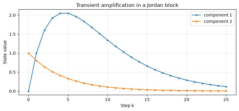
The $2\times2$ block of No.045 is $J=\lambda I+N$ and $N^2=0$. Therefore, $J^k=\lambda^k I+k\lambda^{k-1}N$ appears, and a term containing $k$ appears. $|\lambda|<1$ will eventually converge, but deviations may increase in the early stages.

$J^k=(\lambda I+N)^k=\lambda^k I+k\lambda^{k-1}N\quad(N^2=0)$

Check with Python

J = C[:2, :2]
x0_j = np.array([0.0, 1.0])
steps = np.arange(0, 26)
trajectory = np.array([np.linalg.matrix_power(J, int(k)) @ x0_j for k in steps])
peak_k = int(steps[np.argmax(np.abs(trajectory[:, 0]))])
print(f"First component peaks at step {peak_k}: {trajectory[peak_k, 0]:.4f}")

fig, ax = plt.subplots(figsize=(8, 3.8))
ax.plot(steps, trajectory[:, 0], marker="o", markersize=3, label="component 1")
ax.plot(steps, trajectory[:, 1], marker="s", markersize=3, label="component 2")
ax.set_title("Transient amplification in a Jordan block")
ax.set_xlabel("Step k"); ax.set_ylabel("State value")
ax.grid(True, alpha=0.3); ax.legend(); fig.tight_layout(); plt.show()

First component peaks at step 5: 2.0480

Reading the results

The eigenvalue is 0.8, which is within a stable range, but the first component first increases before decaying. This is because the chain from the second ingredient to the first ingredient works as a $k\lambda^{k-1}$. The allowable upper limit during equipment commissioning must be designed not only for final stability but also for this transient peak.

No.049: Spectral Decomposition

Meaning in Practice

Spectral decomposition of symmetric matrices represents inter-process effects as the addition of orthogonal modes. The contribution of each mode can be visualized individually, making it easier to explain which variation structures are suppressed by improvement measures.

Approach to Analysis and Modeling

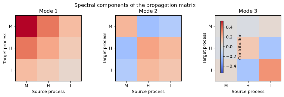
In symmetric matrices, the orthonormal eigenvector $\mathbf{v}_i$ is used and can be decomposed to $A=\sum_i\lambda_i\mathbf{v}_i\mathbf{v}_i^\mathsf{T}$. $\mathbf{v}_i\mathbf{v}_i^\mathsf{T}$ is a projection into that mode. If you leave only the higher modes, it becomes a low-rank approximation.

$A=V\Lambda V^\mathsf{T}=\sum_{i=1}^n\lambda_i\mathbf{v}_i\mathbf{v}_i^\mathsf{T}$

Check with Python

components = [eigvals[i] * np.outer(eigvecs[:, i], eigvecs[:, i]) for i in range(3)]
A_rank1 = components[0]
relative_error = np.linalg.norm(A - A_rank1, "fro") / np.linalg.norm(A, "fro")
display(pd.DataFrame(A_rank1, index=processes, columns=processes).round(3))
print(f"Rank-1 relative Frobenius error = {relative_error:.3f}")

fig, axes = plt.subplots(1, 3, figsize=(10, 3))
vmax = max(np.max(np.abs(c)) for c in components)
for i, (ax, comp) in enumerate(zip(axes, components), 1):
    im = ax.imshow(comp, cmap="coolwarm", vmin=-vmax, vmax=vmax)
    ax.set_title(f"Mode {i}"); ax.set_xlabel("Source process"); ax.set_ylabel("Target process")
    ax.set_xticks(range(3), ["M", "H", "I"]); ax.set_yticks(range(3), ["M", "H", "I"])
    ax.grid(False)
fig.colorbar(im, ax=axes, shrink=0.75, label="Contribution")
fig.suptitle("Spectral components of the propagation matrix")
fig.tight_layout(); plt.show()

	Machining	HeatTreat	Inspection
Machining	0.535	0.349	0.161
HeatTreat	0.349	0.227	0.105
Inspection	0.161	0.105	0.048

Rank-1 relative Frobenius error = 0.643


/var/folders/3y/fmw40k0x78xblvb3gkcyvy1h0000gn/T/ipykernel_35217/1914797165.py:16: UserWarning: This figure includes Axes that are not compatible with tight_layout, so results might be incorrect.
  fig.tight_layout(); plt.show()

Reading the results

Mode 1 contributes in the same direction throughout all processes and remains as a common variation. However, since the relative error of rank 1 approximation cannot be ignored, using only the top 1 mode for practical prediction is too crude. It is effective to use higher-level modes for visualization and explanation, and several modes that meet the required accuracy for control calculations.

No.050: Positive Definite Matrix

Meaning in Practice

When a positive constant-value matrix combines multiple quality deviations into a single loss score, it always imposes a positive penalty on deviations other than zero. Additionally, it makes the quadratic optimization solution unique, enabling stable calculations such as Cholesky decomposition.

Approach to Analysis and Modeling

A symmetric matrix $Q$ is positive definite when it satisfies $\mathbf{x}^\mathsf{T}Q\mathbf{x}>0$ for all nonzero $\mathbf{x}$. In symmetric matrices, it is equivalent to having all eigenvalues being positive. Here, we construct a loss matrix that considers the correlation of quality deviation.

$L(\mathbf{x})=\mathbf{x}^\mathsf{T}Q\mathbf{x},\qquad Q\succ0\Longleftrightarrow\lambda_{\min}(Q)>0$

Check with Python

Q = np.array([[2.0, 0.35, 0.10],
              [0.35, 1.5, 0.25],
              [0.10, 0.25, 1.0]])
q_eigs = np.linalg.eigvalsh(Q)
loss = np.einsum("ij,jk,ik->i", states, Q, states)
print("Eigenvalues of Q:", q_eigs)
print("Positive definite:", np.all(q_eigs > 0))
print(f"Minimum observed loss = {loss.min():.6f}")
display(pd.DataFrame({"Day": quality_df["Day"].head(8), "Quality loss": loss[:8]}).round(4))

fig, ax = plt.subplots(figsize=(8, 3.6))
ax.plot(quality_df["Day"], loss, color="#59A14F")
ax.set_title("Quadratic quality loss over time")
ax.set_xlabel("Day"); ax.set_ylabel("Quality loss x^T Q x")
ax.grid(True, alpha=0.3); fig.tight_layout(); plt.show()

Eigenvalues of Q: [0.8946 1.3903 2.2151]
Positive definite: True
Minimum observed loss = 0.002225

	Day	Quality loss
0	1	6.6620
1	2	3.4683
2	3	2.2214
3	4	1.5221
4	5	1.2650
5	6	0.6545
6	7	0.4485
7	8	0.5211

Reading the results

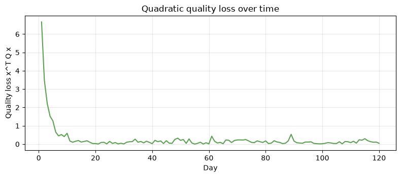
All eigenvalues of $Q$ are positive, and observed losses are non-negative. Therefore, zero deviation is the only minimum point, and the direction of improvement is not ambiguous. However, the weight of $Q$ cannot be determined by mathematics alone. Version management must reflect defect costs, safety impacts, and customer specifications, and be managed with interdepartmental agreement.

Practical Implications Seen Through Target Exercise

In this matrice, the maximum eigenvalue is less than 1, and if there is no disturbance, the quality deviation will converge. However, since control modes spread to multiple processes centered on processing and heat treatment, countermeasures for individual processes alone are likely to recur. Also, as the example of the Jordan block shows, temporary amplification can occur even when eigenvalues are within a stable range.

In practice, the following order is effective.

1. Confirming long-term convergence by spectral radius
2. Narrow down cross-sectional research targets by governing specific vectors
3. Checking overlap and diagonalizability, and evaluating transient responses
4. For symmetric matrices, the contribution by mode is explained using spectral decomposition.
5. Verify that the weight matrix for quality loss is a positive constant value and ensure the uniqueness of optimization.

What is necessary for practical implementation

• Data definition: Standardize measurement units, sampling times, handling missing measurements and outliers, and product variety switching
• Model identification:$A$ is not set as a fixed value, but is estimated from historical data and verified during the holdout period.
• Uncertainty Assessment: In addition to estimating eigenvalues and eigenvectors, we also check the range of fluctuations using bootstraps and similar methods.
• Responding to Non-Steadiness: Monitor equipment maintenance, mold replacement, season, and material lot to ensure lines change
• Causal Verification: The eigenmode is a summary of the correlation structure, and before countermeasures, it is cross-checked with field knowledge, experimental design, and change history.
• Operations Design: Define reestimation frequency, alarm thresholds, approvers, rollback procedures, and model versions

Conclusion

From Articles No.041 to No.050, we confirmed, in a continuous sequence, from eigenvalue analysis that divides matrix repetition actions into “magnification” and “direction,” to the Jordan standard form when diagonalization is non-possible, and positive definite matrices supporting secondary evaluation. Eigenvalues correspond to stability, eigenvectors to the process configuration of fluctuations, redundancy and minimal polynomials to dynamic structures, spectral decomposition to explainability, and positive fixability to validity for evaluation and optimization.

When applying to real data, it is important not to immediately dismiss calculation results as the “cause” but to combine process knowledge with verification experiments.

Consultations for Corporations

At Mathematical Laboratory, we support structural analysis of quality fluctuations using manufacturing data, equipment condition models, anomaly detection, mathematical optimization, and the design of on-site training. You can consult from stages such as “We have data but can’t explain it across processes” or “We want to connect the model to on-site decision-making.”

📩 Contact Us: surikobo.co.jp/contact
Please feel free to consult us first.