Connecting Factory Data to Decision-Making Through ‘Forecasting, Structure, and Time Series’ — 100 Exercises on Linear Algebra in Manufacturing No.081–No.090

Not only quality prediction, but also process networks, similarity searches, and sequential estimation of equipment status are all connected through the common language of linear algebra. Using a fictional precision parts factory as the subject, we implement Linear regression,Ridge Return,PCA、PageRank, Grafflapracian,GCN、Attention, embedded vectors, state-space models, Kalman filters and check “which decisions can be used.”

[!NOTE] This material is a notebook previously used by Surikoubo (or personally by the representative, Kazuyama), and has been reconstructed, edited, and published with the company’s permission. All data listed is fictional and has no relation whatsoever to real companies, factories, or figures.

Introduction: Practical Challenges in Manufacturing Covered in This Article

The target is a precision parts line consisting of processing, heat treatment, polishing, and inspection. On site, predicting quality values, summarizing correlated sensors, identifying critical processes, searching for similar anomalies, and estimating equipment condition including noise all present as separate challenges. However, many of these have the same structure: “converting vectors into matrices” and “extracting important directions.”

Common situations on site

• Although the number of sensors increased, multicollinearity made the regression coefficient unstable.
• Equipment prioritization that ignores inter-process connections overlooks ripple effects.
• Threshold determination is based on time-series measurements as is, increasing false alarms and missed moments
• AI similarity and attention are not explained as on-site decision-making rules.

Why is this issue so difficult to judge?

Correlation is not causation, nor is network importance itself the cause of the defect. Additionally, the observations contain noise, so the true state of the equipment is not directly visible. Rather than taking the output of the mathematical model as a conclusion, it is necessary to make judgments by combining assumptions, verification methods, and operational losses.

Overview of Exercise covered this time

No.081–083 covers prediction and summarization of quality data, No.084–086 covers process networks, No.087–088 covers vector representations of relationships and meanings, and No.089–090 deals with dynamic estimation of equipment condition.

Preparing the Python environment

We use NumPy, pandas, scikit-learn, and Matplotlib. It does not depend on external data and fixes random number seeds. Graph labels are displayed in English to avoid garbled text caused by environmental differences.

import sys
import numpy as np
import pandas as pd
import matplotlib
import matplotlib.pyplot as plt
from IPython.display import display
from sklearn.linear_model import LinearRegression, Ridge
from sklearn.decomposition import PCA
from sklearn.metrics import mean_squared_error
from sklearn.preprocessing import StandardScaler

rng = np.random.default_rng(20260712)
np.set_printoptions(precision=4, suppress=True)
print(f"Python {sys.version.split()[0]}, NumPy {np.__version__}, pandas {pd.__version__}")
print(f"Matplotlib {matplotlib.__version__}")

Python 3.13.1, NumPy 2.5.1, pandas 3.0.3
Matplotlib 3.11.0

Creation of Fictional Data

For 300 lots, we generate cutting speed, feed rate, temperature, vibration, tool wear, and the dimensional deviation (μm) as the target variable. Temperature and vibration share a common factor of equipment load, reproducing correlations that are likely to occur in field data. In the latter half, we also use the four-stage directed network and equipment status at 60 o’clock.

n = 300
load = rng.normal(0, 1, n)
speed = rng.normal(120, 8, n)
feed = rng.normal(0.24, 0.025, n)
temperature = 68 + 4.5 * load + rng.normal(0, 1.2, n)
vibration = 2.2 + 0.38 * load + rng.normal(0, 0.12, n)
wear = rng.uniform(0, 1, n)
deviation = (0.055 * (speed - 120) + 8.0 * (feed - 0.24)
             + 0.16 * (temperature - 68) + 0.85 * wear
             + rng.normal(0, 0.32, n))
df = pd.DataFrame({"speed": speed, "feed": feed, "temperature": temperature,
                   "vibration": vibration, "wear": wear, "deviation_um": deviation})
display(df.head().round(3))
display(df.describe().loc[["mean", "std", "min", "max"]].round(3))

	speed	feed	temperature	vibration	wear	deviation_um
0	113.914	0.200	72.476	2.813	0.057	0.303
1	119.946	0.234	71.160	2.337	0.521	1.161
2	113.412	0.254	70.924	2.586	0.985	0.638
3	117.380	0.231	68.729	2.360	0.541	0.325
4	120.078	0.270	70.845	2.498	0.979	1.651

	speed	feed	temperature	vibration	wear	deviation_um
mean	119.495	0.240	67.847	2.200	0.493	0.343
std	7.634	0.025	4.731	0.403	0.290	0.970
min	96.994	0.168	52.460	0.913	0.000	-2.156
max	144.210	0.312	82.143	3.521	0.998	3.391

No.081: Linear Regression

Meaning in Practice

Dimensional deviations can be predicted from multiple processing conditions, and the average change when the condition is changed by one unit can be explained as a coefficient.

Approach to Analysis and Modeling

Place $\mathbf{y}=X\boldsymbol{\beta}+\boldsymbol{\varepsilon}$ and find the coefficients using least squares $\min_{\beta}\|\mathbf{y}-X\boldsymbol{\beta}\|_2^2$. Causal interpretation of coefficients requires separate verification of confounding, nonlinearity, and operating range.

Check with Python

features = ["speed", "feed", "temperature", "vibration", "wear"]
train = np.arange(0, 220); test = np.arange(220, n)
X, y = df[features].to_numpy(), df["deviation_um"].to_numpy()
lr = LinearRegression().fit(X[train], y[train])
pred_lr = lr.predict(X[test])
coef_lr = pd.DataFrame({"feature": features, "coefficient": lr.coef_})
display(coef_lr.round(4))
print(f"Test RMSE: {mean_squared_error(y[test], pred_lr)**0.5:.3f} µm")
plt.figure(figsize=(6, 4)); plt.scatter(y[test], pred_lr, alpha=.65)
lims=[y[test].min(), y[test].max()]; plt.plot(lims, lims, '--', color='black')
plt.title("Measured vs predicted deviation"); plt.xlabel("Measured deviation (µm)"); plt.ylabel("Predicted deviation (µm)")
plt.grid(alpha=.3); plt.tight_layout(); plt.show()

	feature	coefficient
0	speed	0.0570
1	feed	6.4424
2	temperature	0.1739
3	vibration	-0.2135
4	wear	0.8640

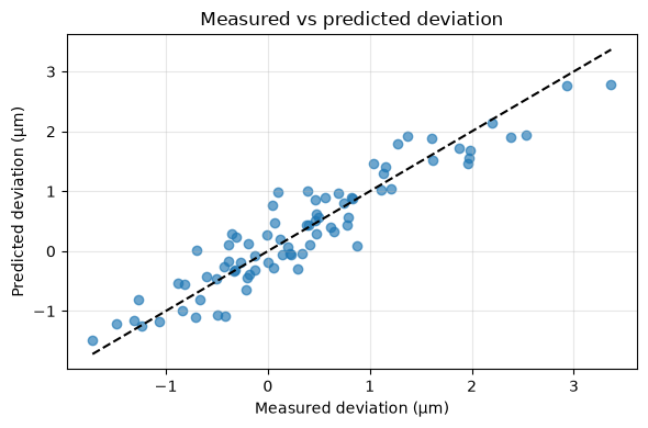
Test RMSE: 0.357 µm

Reading the results

Forecasts are concentrated around the 45th parallel, capturing average quality fluctuations. Since coefficients differ in units, importance comparison cannot be made using only absolute values. Residuals are checked by variety, equipment, and timing, and acceptance is determined based on whether the RMSE is sufficiently small compared to the current management range.

No.082: Ridge Returns

Meaning in Practice

When there are many correlated sensors, the coefficient codes and sizes fluctuate with each data update. Ridge stabilizes coefficients while maintaining forecast accuracy.

Approach to Analysis and Modeling

$\min_{\beta}\|\mathbf{y}-X\boldsymbol{\beta}\|_2^2+\alpha\|\boldsymbol{\beta}\|_2^2$ and penalties are added. After standardization, $\alpha$ are compared and selected based on unused periods or cross-validation.

Check with Python

scaler = StandardScaler().fit(X[train])
Xs_train, Xs_test = scaler.transform(X[train]), scaler.transform(X[test])
rows=[]
for alpha in [0, 0.1, 1, 10, 100]:
    model = Ridge(alpha=alpha).fit(Xs_train, y[train])
    rows.append([alpha, mean_squared_error(y[test], model.predict(Xs_test))**0.5,
                 np.linalg.norm(model.coef_)])
ridge_result = pd.DataFrame(rows, columns=["alpha", "test_RMSE", "coefficient_L2_norm"])
display(ridge_result.round(4))
best_alpha = ridge_result.loc[ridge_result.test_RMSE.idxmin(), "alpha"]
ridge = Ridge(alpha=best_alpha).fit(Xs_train, y[train])
display(pd.DataFrame({"feature":features, "standardized_coefficient":ridge.coef_}).round(4))

	alpha	test_RMSE	coefficient_L2_norm
0	0.0	0.3573	0.9524
1	0.1	0.3572	0.9499
2	1.0	0.3561	0.9288
3	10.0	0.3554	0.8020
4	100.0	0.4334	0.5515

	feature	standardized_coefficient
0	speed	0.4015
1	feed	0.1558
2	temperature	0.6299
3	vibration	0.0674
4	wear	0.2376

Reading the results

Stricter penalties shrink the coefficient norm, but too much worsens RMSE. Since the selection depends on the current split, we use chronological verification in production. While stable coefficients are easy to explain, Ridge does not strictly zero unnecessary variables.

No.083: Dimension Reduction by PCA

Meaning in Practice

Numerous correlation sensors are compressed into a few composite axes for “equipment load” and “processing conditions,” organizing monitoring screens and abnormal trends.

Approach to Analysis and Modeling

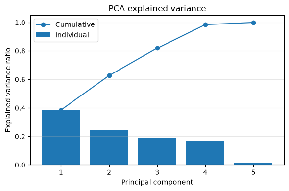
Normalized matrix $Z$ is determined as the eigenvector in which the orthogonal direction maximizes variance. $k$ The variance of the principal component is the corresponding eigenvalue. PCA is unsupervised and may abandon the low-dispersion direction that is important for quality.

Check with Python

Z = StandardScaler().fit_transform(df[features])
pca = PCA().fit(Z)
scores = pca.transform(Z)
cum = np.cumsum(pca.explained_variance_ratio_)
display(pd.DataFrame({"PC":np.arange(1,6), "explained_ratio":pca.explained_variance_ratio_, "cumulative":cum}).round(3))
display(pd.DataFrame(pca.components_[:2], index=["PC1","PC2"], columns=features).round(3))
plt.figure(figsize=(6,4)); plt.bar(np.arange(1,6), pca.explained_variance_ratio_, label="Individual")
plt.plot(np.arange(1,6), cum, marker='o', label="Cumulative")
plt.title("PCA explained variance"); plt.xlabel("Principal component"); plt.ylabel("Explained variance ratio")
plt.grid(axis='y', alpha=.3); plt.legend(); plt.tight_layout(); plt.show()

	PC	explained_ratio	cumulative
0	1	0.385	0.385
1	2	0.242	0.627
2	3	0.192	0.819
3	4	0.166	0.985
4	5	0.015	1.000

	speed	feed	temperature	vibration	wear
PC1	0.039	0.027	0.706	0.706	-0.008
PC2	-0.401	0.630	0.012	-0.006	0.665

Reading the results

You can select the number of components based on the cumulative contribution rate and the required information retention rate. Looking at the load, temperature and vibration greatly contribute to the same main component, suggesting the existence of a common load. However, naming the main component is hypothetical and is supported by conservation records and experiments.

No.084：PageRank

Meaning in Practice

From the abnormal ripple network between processes, monitoring priorities are assigned, including not only the number of direct connections but also “processes affected by critical processes.”

Approach to Analysis and Modeling

For column probability matrices $P$, iteratively compute $\mathbf{r}=dP\mathbf{r}+(1-d)\mathbf{1}/n$ steady solutions. The edge is defined as the causal ripple direction and the damping coefficient $d$ suppresses concentration in the cycle.

Check with Python

processes = ["Machining", "HeatTreat", "Polishing", "Inspection"]
# A[i,j]: process j influences process i
A = np.array([[0,0,0,0.2], [0.8,0,0,0], [0.2,0.7,0,0], [0,0.3,1.0,0]], float)
P = A / A.sum(axis=0, keepdims=True)
r = np.ones(4)/4; d=.85
for _ in range(100): r = d * P @ r + (1-d)/4
rank_df = pd.DataFrame({"process":processes, "PageRank":r}).sort_values("PageRank", ascending=False)
display(rank_df.round(4))
plt.figure(figsize=(6,4)); plt.bar(rank_df.process, rank_df.PageRank)
plt.title("Process propagation priority by PageRank"); plt.xlabel("Process"); plt.ylabel("PageRank score")
plt.grid(axis='y', alpha=.3); plt.xticks(rotation=20); plt.tight_layout(); plt.show()

	process	PageRank
3	Inspection	0.2805
0	Machining	0.2760
1	HeatTreat	0.2251
2	Polishing	0.2184

Reading the results

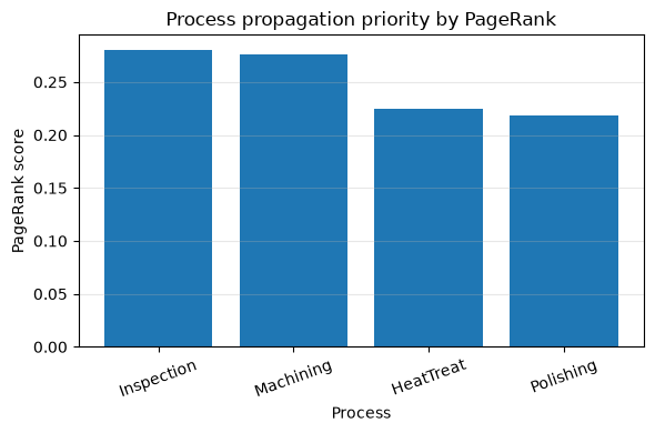
High-score processes are key monitoring candidates for ripple structures. However, since PageRank does not include defect rates, downtime losses, or detectability, it is integrated with risk indicators such as FMEA to determine maintenance priorities.

No.085: Grafflaplasian

Meaning in Practice

It is possible to detect significantly different sensor values between adjacent equipment and to divide lines into groups based on process and equipment connections.

Approach to Analysis and Modeling

For undirected weighted matrices $W$ and degree matrices $D$, $L=D-W$ is the . $\mathbf{x}^\mathsf{T}L\mathbf{x}=\frac12\sum_{ij}w_{ij}(x_i-x_j)^2$ measures discrepancies between adjacent nodes. The second eigenvector provides clues for splitting.

Check with Python

W = (A + A.T) / 2
D = np.diag(W.sum(axis=1)); L = D - W
evals, evecs = np.linalg.eigh(L)
temp_normal = np.array([68.0, 69.0, 70.0, 69.5])
temp_alarm = np.array([68.0, 77.0, 70.0, 69.5])
energy = lambda x: float(x @ L @ x)
display(pd.DataFrame(L, index=processes, columns=processes).round(2))
print("Eigenvalues:", evals.round(4))
print(f"Smoothness normal={energy(temp_normal):.2f}, alarm={energy(temp_alarm):.2f}")

	Machining	HeatTreat	Polishing	Inspection
Machining	0.6	-0.40	-0.10	-0.10
HeatTreat	-0.4	0.90	-0.35	-0.15
Polishing	-0.1	-0.35	0.95	-0.50
Inspection	-0.1	-0.15	-0.50	0.75

Eigenvalues: [0.     0.6032 1.141  1.4557]
Smoothness normal=1.54, alarm=58.74

Reading the results

Zero eigenvalues correspond to a constant value across the entire network. In cases where only the heat treatment temperature was raised, the Laplacian secondary form increased, allowing detection of local mismatches from the perspective of connection relationships. The normal range and the appropriateness of side weights for each process determine operational accuracy.

No.086：GCN

Meaning in Practice

Not only the sensor characteristics of each piece of equipment but also information from connected equipment are mixed together for anomaly detection and failure prediction.

Approach to Analysis and Modeling

Using $\tilde A=A+I$ and $\tilde D$ with self-looping, the first layer is represented as $H'=\sigma(\tilde D^{-1/2}\tilde A\tilde D^{-1/2}HW)$. Here, we examine feature smoothing through propagation rather than learning.

Check with Python

A_u = (W > 0).astype(float); A_tilde = A_u + np.eye(4)
D_inv_sqrt = np.diag(1 / np.sqrt(A_tilde.sum(axis=1)))
A_norm = D_inv_sqrt @ A_tilde @ D_inv_sqrt
H = np.array([[1.8,68], [3.4,76], [2.0,70], [1.5,69]], float)
H_scaled = StandardScaler().fit_transform(H)
H_gcn = np.maximum(0, A_norm @ H_scaled @ np.array([[.8,.2],[.2,.8]]))
display(pd.DataFrame(H_scaled, index=processes, columns=["vibration_z","temperature_z"]).round(3))
display(pd.DataFrame(H_gcn, index=processes, columns=["GCN_feature_1","GCN_feature_2"]).round(3))

	vibration_z	temperature_z
Machining	-0.514	-0.884
HeatTreat	1.680	1.687
Polishing	-0.240	-0.241
Inspection	-0.926	-0.562

	GCN_feature_1	GCN_feature_2
Machining	0.0	0.0
HeatTreat	0.0	0.0
Polishing	0.0	0.0
Inspection	0.0	0.0

Reading the results

The high-temperature characteristics of heat treatment are transmitted to adjacent processes, representing ambient effects that cannot be seen by a standalone sensor. If you stack too many layers, over-smoothing occurs where all equipment is similar, so performance is verified by time series segmentation, and the graph is updated when equipment connections change.

No.087: Attention of Transformers

Meaning in Practice

When an abnormality occurs, you can use weights to determine which past operating points are strongly referenced to create the current expression.

Approach to Analysis and Modeling

$\mathrm{Attention}(Q,K,V)=\mathrm{softmax}(QK^\mathsf{T}/\sqrt{d_k})V$ is here. Similarity is converted into probabilistic weights, but weights do not automatically guarantee causal contribution or accountability.

Check with Python

X_seq = np.array([[0.1,0.2], [0.2,0.1], [1.6,1.3], [0.3,0.2], [1.4,1.1]])
Q=K=V=X_seq; logits = Q @ K.T / np.sqrt(2)
logits -= logits.max(axis=1, keepdims=True)
weights = np.exp(logits); weights /= weights.sum(axis=1, keepdims=True)
context = weights @ V
display(pd.DataFrame(weights, index=[f"query_t{i}" for i in range(5)], columns=[f"key_t{i}" for i in range(5)]).round(3))
plt.figure(figsize=(6,4)); plt.imshow(weights, cmap="Blues", aspect="auto"); plt.colorbar(label="Attention weight")
plt.title("Scaled dot-product attention"); plt.xlabel("Key time"); plt.ylabel("Query time"); plt.grid(False); plt.tight_layout(); plt.show()

	key_t0	key_t1	key_t2	key_t3	key_t4
query_t0	0.180	0.179	0.234	0.183	0.224
query_t1	0.177	0.178	0.236	0.182	0.227
query_t2	0.035	0.036	0.531	0.044	0.353
query_t3	0.163	0.164	0.261	0.170	0.243
query_t4	0.048	0.049	0.496	0.058	0.349

Reading the results

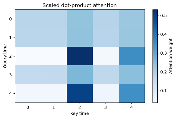
Periods of high load place significant weight on similarly high-load past moments. In practice, masking, location information, multiple heads, and trained projections are added. Attention does not definitively determine the cause through visualization alone; instead, it verifies through input perturbations and on-site records.

No.088: Embedding Vector

Meaning in Practice

Conversion of maintenance records and abnormal patterns into low-dimensional vectors allows you to search for similar past cases and countermeasures.

Approach to Analysis and Modeling

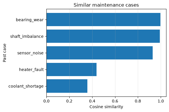
Cosine similarity $\cos(\theta)=\mathbf{a}^\mathsf{T}\mathbf{b}/(\|\mathbf{a}\|\|\mathbf{b}\|)$ measures the proximity of direction. Here, we use explainable fictitious embeddings to check the search mechanism.

Check with Python

labels = ["bearing_wear", "shaft_imbalance", "coolant_shortage", "heater_fault", "sensor_noise"]
E = np.array([[.9,.7,.1], [.8,.9,.1], [.2,.1,.9], [.1,.3,.8], [.4,.2,.2]])
query = np.array([.85,.75,.15])
cos = (E @ query) / (np.linalg.norm(E,axis=1)*np.linalg.norm(query))
search = pd.DataFrame({"past_case":labels, "cosine_similarity":cos}).sort_values("cosine_similarity", ascending=False)
display(search.round(3))
plt.figure(figsize=(6,4)); plt.barh(search.past_case[::-1], search.cosine_similarity[::-1])
plt.title("Similar maintenance cases"); plt.xlabel("Cosine similarity"); plt.ylabel("Past case")
plt.grid(axis='x', alpha=.3); plt.tight_layout(); plt.show()

	past_case	cosine_similarity
0	bearing_wear	0.997
1	shaft_imbalance	0.992
4	sensor_noise	0.928
3	heater_fault	0.437
2	coolant_shortage	0.358

Reading the results

Examples of bearing wear and shaft misalignment close to the inquiry vector have become top-ranked. Search accuracy depends on embedded models, recording quality, and thresholds. Access control for confidential information and operations where experts approve search results are required.

No.089: State Space Model

Meaning in Practice

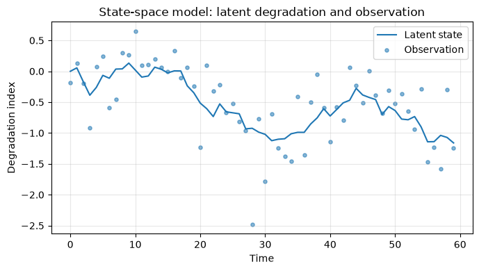
We express the true state of equipment deterioration, which is not directly visible, by dividing it into time evolution and sensor observations, creating a common blueprint for predictive maintenance.

Approach to Analysis and Modeling

$\mathbf{x}_t=F\mathbf{x}_{t-1}+\mathbf{w}_t$, let $\mathbf{y}_t=H\mathbf{x}_t+\mathbf{v}_t$, $F$ be the state transition, and $H$ is the observation matrix. Process noise $Q$ and observation noise $R$ represent the confidence in the model and measurement.

Check with Python

T=60; F=np.array([[1,.08],[0,1]]); H=np.array([[1,0]])
Q=np.diag([.015,.003]); R=np.array([[.18]])
x_true=np.zeros((T,2)); y_obs=np.zeros(T); x_true[0]=[0,.04]
for t in range(1,T): x_true[t]=F@x_true[t-1]+rng.multivariate_normal([0,0],Q)
for t in range(T): y_obs[t]=(H@x_true[t])[0]+rng.normal(0,np.sqrt(R[0,0]))
display(pd.DataFrame({"time":np.arange(6), "latent_degradation":x_true[:6,0], "observed_sensor":y_obs[:6]}).round(3))
plt.figure(figsize=(7,4)); plt.plot(x_true[:,0], label="Latent state"); plt.scatter(range(T),y_obs,s=14,alpha=.55,label="Observation")
plt.title("State-space model: latent degradation and observation"); plt.xlabel("Time"); plt.ylabel("Degradation index")
plt.grid(alpha=.3); plt.legend(); plt.tight_layout(); plt.show()

	time	latent_degradation	observed_sensor
0	0	0.000	-0.186
1	1	0.055	0.134
2	2	-0.171	-0.196
3	3	-0.388	-0.915
4	4	-0.262	0.077
5	5	-0.066	0.244

Reading the results

Observed values fluctuate significantly around the true degradation state, and simple thresholds can lead to false alarms. The main challenges are defining states, sampling intervals, and identifying $F,H,Q,R$. After equipment upgrades or changes in operating conditions, the estimate will be reconsidered.

No.090: Karman Filter

Meaning in Practice

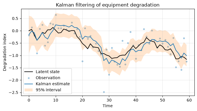
Based on state-space models, forecasting and observation are sequentially integrated according to uncertainty. Smooth degradation estimation and confidence intervals stabilize conservation decisions.

Approach to Analysis and Modeling

Forecasts $\hat x_t^-=F\hat x_{t-1}$ and updates $\hat x_t=\hat x_t^-+K_t(y_t-H\hat x_t^-)$ repeatedly. $K_t=P_t^-H^\mathsf{T}(HP_t^-H^\mathsf{T}+R)^{-1}$ determines the weight of predictions and observations.

Check with Python

xhat=np.zeros(2); P=np.eye(2); estimates=[]; sigmas=[]; gains=[]
for yt in y_obs:
    xp=F@xhat; Pp=F@P@F.T+Q
    S=H@Pp@H.T+R; K=Pp@H.T@np.linalg.inv(S)
    xhat=xp+(K[:,0]*(yt-(H@xp)[0])); P=(np.eye(2)-K@H)@Pp
    estimates.append(xhat.copy()); sigmas.append(np.sqrt(P[0,0])); gains.append(K[0,0])
estimates=np.array(estimates); sigmas=np.array(sigmas)
rmse_obs=np.sqrt(np.mean((y_obs-x_true[:,0])**2)); rmse_kf=np.sqrt(np.mean((estimates[:,0]-x_true[:,0])**2))
print(f"Observation RMSE={rmse_obs:.3f}, Kalman estimate RMSE={rmse_kf:.3f}, final gain={gains[-1]:.3f}")
plt.figure(figsize=(7,4)); plt.plot(x_true[:,0],label="Latent state",color="black"); plt.scatter(range(T),y_obs,s=12,alpha=.35,label="Observation")
plt.plot(estimates[:,0],label="Kalman estimate"); plt.fill_between(range(T),estimates[:,0]-1.96*sigmas,estimates[:,0]+1.96*sigmas,alpha=.2,label="95% interval")
plt.title("Kalman filtering of equipment degradation"); plt.xlabel("Time"); plt.ylabel("Degradation index")
plt.grid(alpha=.3); plt.legend(); plt.tight_layout(); plt.show()

Observation RMSE=0.412, Kalman estimate RMSE=0.225, final gain=0.276

Reading the results

The Kalman estimate was closer to the true state than raw observations and also provided confidence intervals. Maintenance orders are reasonable not only when the estimated value exceeds the threshold, but also by combining the probability of exceeding the threshold within a certain period with stoppage losses. Since linear and Gaussian assumptions do not apply to sudden failure changes, residual monitoring and other abnormality detection methods are used together.

Practical Implications Seen Through Target Exercise

The 10 techniques are not separate buzzwords. Regression is a linear mapping from features to quality, PCA is projection in the critical direction, PageRank and Laplacian are matrixed process connections, GCN and Attention are information aggregation according to relationships, and state-space models and Karman filters are matrix transformations in the time direction.

In practice, decisions and losses are first determined, then matrices are designed to fit the data generation process, and finally validated after unused periods, different equipment, and condition changes. Using explainable small-scale models as a baseline allows you to measure the added value of advanced models.

What is necessary for practical implementation

1. Agree on objective KPIs, decision deadlines, and costs for false alarms or missed reports
2. Maintain sensor calibration, missing units, equipment, and product master systems
3. Conducting timeline verification and comparative testing with current rules
4. Manage models, thresholds, graphs, and training data
5. Establish operational responsibilities including on-site approval, monitoring, relearning, and stoppage decisions

Conclusion

Linear algebra is a practical language for considering quality prediction, process structure, similarity search, and dynamic estimation within the same framework. The key to advancing PoC operations is not only the calculation results but also clearly indicating what each element of the matrix means and under which assumptions it can be used for decision-making.

Consultations for Corporations

At Mathematical Laboratory, we support you according to your challenges and data maturity, covering everything from manufacturing data diagnosis, quality prediction, equipment maintenance, process network analysis, to AI and mathematical model training and implementation.

📩 Contact Us: surikobo.co.jp/contact Please feel free to consult us first.