Compatibility Completion × Equipment Varieties and Large-Scale Process Calculations — 100 Exercises on Linear Algebra in Manufacturing No.071–No.080

In multi-product production, it is impossible to prototype all combinations of equipment and varieties. On the other hand, daily production planning and equipment condition design involve handling large queues with unevaluated combinations and needing to get answers within limited time. In this article, we use product data × fictional equipment to link Recommendations through matrix decomposition, latent factors,Truncated / Randomized SVD、Krylov Partial space method,Arnoldi Method, conjugate gradient method, preprocessing, sparse matrix solver, large-scale matrix computation to decision-making at the manufacturing floor.

[!NOTE] This material is a notebook previously used by Surikoubo (or personally by the representative, Kazuyama), and has been reconstructed, edited, and published with the company’s permission.
All data listed is fictional and has no relation whatsoever to real companies, factories, or figures.

Introduction: Practical Challenges in Manufacturing Covered in This Article

Consider a line that processes 18 types of equipment with 12 machines. In prototype combinations, the “degree of fit” by integrating yield rate, setup time, and energy intensity can be identified, but most of these are not evaluated. In the first half of this paper, we estimate the preferred candidates for unevaluated combinations based on observed evaluations. In the second half, we efficiently solve linear equations of large-scale temperature fields generated in the same factory using sparse matrices and iterative methods.

Common situations on site

• We assign equipment × types without proven track record based solely on the experience of the person in charge
• Comprehensive combination testing cannot be conducted in terms of time, materials, and stoppage losses.
• Finely refine the simulation meshes cause a sharp increase in computation time and memory
• Even if a solution is obtained, errors, convergence conditions, and candidate selection rules are not managed

Why is this issue so difficult to judge?

Unobserved is not ‘non-compliant,’ but ‘not yet tested.’ Also, the scores of low-rank models are not causal effects or safety guarantees. On a computational side, explicitly creating a huge dense matrix will drain memory first. Accuracy, computational cost, explainability, and safety constraints must be addressed simultaneously.

Overview of Exercise covered this time

In No.071–074, we create low-rank models that recommend equipment candidates, and in No.075–080, we proceed to the method of ‘calculating only the necessary parts’ for large-scale linear calculations. The first half is centered on Priority for Exploring Combinations, while the second half centers on How to return a reliable numerical solution within the constraint time limit.

Preparing the Python environment

NumPy and pandas handle calculations and table creation, Matplotlib visualization, SciPy for sparse matrices and iteration, and scikit-learn for Randomized SVD. Fix the random number seed and make it reexecutable.

import sys, time
import numpy as np
import pandas as pd
import matplotlib
import matplotlib.pyplot as plt
from IPython.display import display
from scipy import sparse
from scipy.sparse.linalg import LinearOperator, cg, eigsh, spsolve
from sklearn.utils.extmath import randomized_svd

rng = np.random.default_rng(71080)
np.set_printoptions(precision=4, suppress=True)
pd.set_option("display.max_columns", 12)
print("Python:", sys.version.split()[0])
print("NumPy:", np.__version__, "| pandas:", pd.__version__)
print("Matplotlib:", matplotlib.__version__)

Python: 3.13.1
NumPy: 2.5.1 | pandas: 3.0.3
Matplotlib: 3.11.0

Creation of Fictional Data

Assume there are three latent axes for equipment capacity and product requirements: precision machining, thermal stability, and mass production suitability. A small measurement noise is added to the true fit, and only about 55% is considered prototype. Missing masks are generated independently of evaluation values, and it is confirmed that each piece of equipment and product has at least one observation.

n_machines, n_products, rank_true = 12, 18, 3
machines = [f"M{i:02d}" for i in range(1, n_machines + 1)]
products = [f"P{i:02d}" for i in range(1, n_products + 1)]
U_true = rng.normal(size=(n_machines, rank_true))
V_true = rng.normal(size=(n_products, rank_true))
raw = U_true @ V_true.T
true_score = 50 + 12 * (raw - raw.mean()) / raw.std()
true_score = np.clip(true_score, 5, 95)
observed_score = np.clip(true_score + rng.normal(0, 2.0, true_score.shape), 0, 100)
mask = rng.random(true_score.shape) < 0.55
for i in range(n_machines): mask[i, rng.integers(n_products)] = True
for j in range(n_products): mask[rng.integers(n_machines), j] = True
R = np.where(mask, observed_score, np.nan)
print(f"Matrix shape: {R.shape}, observed: {mask.sum()}/{R.size} ({mask.mean():.1%})")
display(pd.DataFrame(R, index=machines, columns=products).iloc[:6, :9].round(1))

Matrix shape: (12, 18), observed: 137/216 (63.4%)

	P01	P02	P03	P04	P05	P06	P07	P08	P09
M01	54.1	NaN	41.2	59.5	49.1	59.3	56.3	NaN	NaN
M02	57.8	59.8	NaN	62.0	59.0	NaN	61.3	58.2	62.4
M03	50.2	46.6	45.9	NaN	51.7	NaN	NaN	51.2	40.1
M04	NaN	61.9	38.8	62.5	72.4	NaN	NaN	60.9	NaN
M05	NaN	NaN	NaN	58.5	40.4	49.1	47.7	53.6	12.7
M06	50.7	48.1	NaN	46.4	38.0	51.4	52.3	45.8	67.4

No.071: Matrix Breakdown of Recommendation Systems

Meaning in Practice

The recommendation system can be used not only for EC products but also as a mechanism to rank combinations with the highest value for prototyping from unevaluated equipment × varieties. It is not intended to automate safety certification, but is used to narrow down the test plan.

Approach to Analysis and Modeling

Let the observation set be $\Omega$, and the low-rank matrix $UV^\top$ reproduce the observations. $\min_{U,V}\sum_{(i,j)\in\Omega}(R_{ij}-\mathbf{u}_i^\top\mathbf{v}_j)^2+\lambda(\|U\|_F^2+\|V\|_F^2)$ Solve using Alternate Least Squares (ALS). Unobserved cells cannot be included in losses.

Check with Python

def als(R, mask, k=3, reg=3.0, epochs=30, seed=1):
    g = np.random.default_rng(seed); m, n = R.shape
    U = g.normal(0, .2, (m, k)); V = g.normal(0, .2, (n, k)); I = np.eye(k)
    for _ in range(epochs):
        for i in range(m):
            js = np.where(mask[i])[0]; U[i] = np.linalg.solve(V[js].T @ V[js] + reg*I, V[js].T @ R[i, js])
        for j in range(n):
            ii = np.where(mask[:, j])[0]; V[j] = np.linalg.solve(U[ii].T @ U[ii] + reg*I, U[ii].T @ R[ii, j])
    return U, V
U, V = als(np.nan_to_num(R), mask)
pred = U @ V.T
candidates = [(pred[i,j], machines[i], products[j]) for i,j in zip(*np.where(~mask))]
top5 = pd.DataFrame(sorted(candidates, reverse=True)[:5], columns=["Predicted score","Machine","Product"])
display(top5.round(1))

	Predicted score	Machine	Product
0	90.6	M12	P10
1	84.2	M12	P09
2	72.1	M06	P03
3	71.5	M12	P03
4	69.8	M09	P02

Reading the results

The top five are not ‘confirmed’ but are prototype candidates. After excluding candidates based on equipment specifications, jig compatibility, and legal and safety conditions, we move on to small-batch prototyping. Not only are scores ranked higher, but uncertainty in predictions and exam costs are also taken into account at the next stage.

No.072：Latent Factor Model

Meaning in Practice

Latent factors are presented by compressing common axes of equipment capacity and product requirements that are not directly recorded in the table. Equipment and types can be arranged with similar trends, serving as an entry point to discuss candidate reasons with engineers.

Approach to Analysis and Modeling

The forecast value $\hat R_{ij}=\mathbf{u}_i^\top\mathbf{v}_j$ is the consumable product of factors on both the equipment side and the product type. However, since the predicted values do not change even after rotation, each axis is not automatically labeled as “stiff,” but interpreted based on correlation with known specifications.

Check with Python

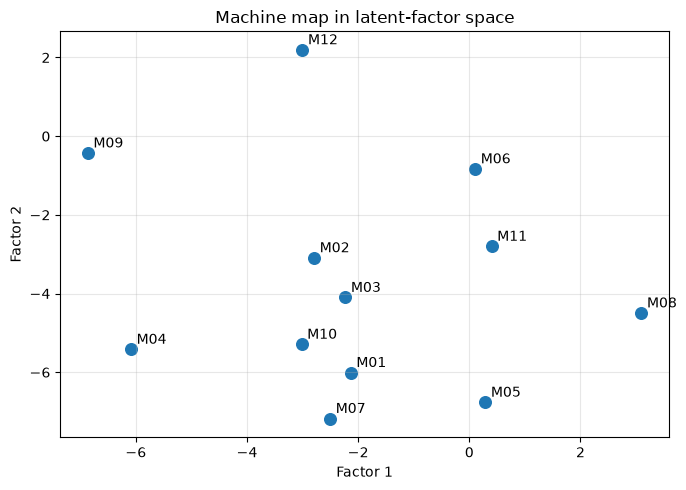
factor_df = pd.DataFrame(U, index=machines, columns=["Factor 1","Factor 2","Factor 3"])
display(factor_df.round(2))
fig, ax = plt.subplots(figsize=(7, 5))
ax.scatter(U[:,0], U[:,1], s=70)
for i, name in enumerate(machines): ax.annotate(name, (U[i,0], U[i,1]), xytext=(4,4), textcoords="offset points")
ax.set_title("Machine map in latent-factor space")
ax.set_xlabel("Factor 1"); ax.set_ylabel("Factor 2"); ax.grid(True, alpha=.3); plt.tight_layout(); plt.show()

	Factor 1	Factor 2	Factor 3
M01	-2.13	-6.01	-7.03
M02	-2.79	-3.09	-9.36
M03	-2.23	-4.10	-7.06
M04	-6.09	-5.42	-6.85
M05	0.29	-6.76	-5.46
M06	0.11	-0.83	-10.22
M07	-2.50	-7.18	-5.65
M08	3.10	-4.49	-6.91
M09	-6.86	-0.43	-9.29
M10	-3.02	-5.29	-6.61
M11	0.40	-2.80	-8.37
M12	-3.00	2.20	-11.07

Reading the results

Facilities placed nearby have observed fit patterns similar to those observed. Verify consistency between factors and known attributes by cross-checking with ledgers such as maintenance methods and spindle specifications. Factor maps are not causal explanations, but maps for comparing equipment groups and conducting additional investigations.

No.073：Truncated SVD

Meaning in Practice

Truncated SVD approximates large evaluation matrices using only the top $k$ components, reducing data volume while preserving key patterns. Since all components are not stored or calculated, prediction and visualization can be lightened.

Approach to Analysis and Modeling

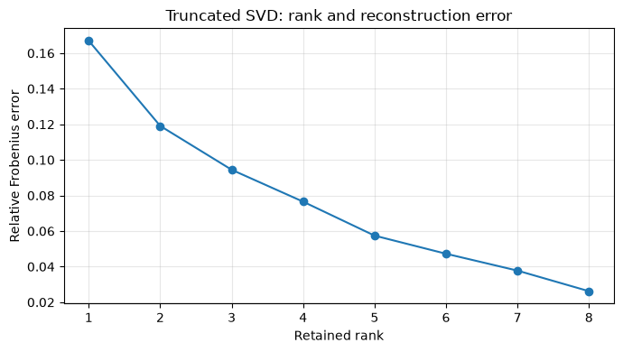
$R\approx U_k\Sigma_kV_k^\top$ is used, and the amount of information retained is evaluated by the square ratio of the singular values. Since SVD is intended for complete matrices, missing measurements are treated here as baselines provisionally supplemented by the variety average, and the difference from ALS is clearly stated.

Check with Python

filled = R.copy(); col_means = np.nanmean(filled, axis=0)
filled[np.where(np.isnan(filled))] = np.take(col_means, np.where(np.isnan(filled))[1])
Uc, s, Vt = np.linalg.svd(filled, full_matrices=False)
errors=[]
for k in range(1, 9):
    approx=(Uc[:,:k]*s[:k])@Vt[:k]
    errors.append(np.linalg.norm(filled-approx,"fro")/np.linalg.norm(filled,"fro"))
display(pd.DataFrame({"rank":range(1,9),"relative_error":errors}).round(4))
fig, ax=plt.subplots(figsize=(7,4)); ax.plot(range(1,9),errors,marker="o")
ax.set_title("Truncated SVD: rank and reconstruction error"); ax.set_xlabel("Retained rank"); ax.set_ylabel("Relative Frobenius error")
ax.grid(True,alpha=.3); plt.tight_layout(); plt.show()

	rank	relative_error
0	1	0.1669
1	2	0.1191
2	3	0.0944
3	4	0.0765
4	5	0.0574
5	6	0.0472
6	7	0.0378
7	8	0.0262

Reading the results

The higher the rank, the lower the reconstruction error, but the more complexity it becomes. Rankings are not determined solely by bending; instead, the prediction error is divided into training and validation of observation data, and the computational time that can be used. If the mean interception is biased in the missing mechanism, systematic errors can occur.

No.074：Randomized SVD

Meaning in Practice

Randomized SVD rapidly approximates the required top-level singular components using probabilistic projections. This is effective when the number of facilities and variety increases and daily retraining time becomes a constraint.

Approach to Analysis and Modeling

Extract the main column space from random matrices and perform SVD on smaller matrices. The seed is fixed to ensure reproducibility, and the difference from the exact SVD is measured using reconstruction errors.

Check with Python

k=3
Ur,sr,Vtr=randomized_svd(filled,n_components=k,n_iter=5,random_state=71080)
rand_approx=(Ur*sr)@Vtr; exact_approx=(Uc[:,:k]*s[:k])@Vt[:k]
comparison=pd.DataFrame({"method":["Exact truncated SVD","Randomized SVD"],
 "relative_error":[np.linalg.norm(filled-exact_approx,"fro")/np.linalg.norm(filled,"fro"),np.linalg.norm(filled-rand_approx,"fro")/np.linalg.norm(filled,"fro")],
 "top_singular_value":[s[0],sr[0]]})
display(comparison.round(6))

	method	relative_error	top_singular_value
0	Exact truncated SVD	0.094438	741.215763
1	Randomized SVD	0.094438	741.215763

Reading the results

Even in small-scale cases, the error of Randomized SVD approaches a strict rank 3 approximation. Since speed differences appear in large-scale data, time and memory are measured at production-equivalent size. Leave operational settings for variations caused by random numbers, number of iterations, and tolerance of error.

No.075: Krylov Fractional Space Method

Meaning in Practice

In temperature field and deformation analysis, it is more practical to repeatedly multiply the matrix and vectors to obtain only the necessary solution and eigenmode rather than decomposing the entire matrix. The Krylov Law is the foundation of this.

Approach to Analysis and Modeling

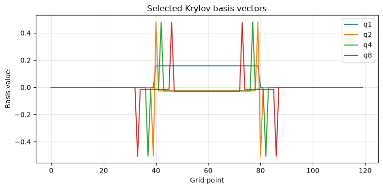
$\mathcal K_m(A,b)=\mathrm{span}\{b,Ab,A^2b,\ldots,A^{m-1}b\}$ is made. Here, we orthogonalize the basis of the discrete matrix of one-dimensional thermal conduction and observe how the subspace expands.

Check with Python

n=120
A_heat=sparse.diags([-np.ones(n-1),2.2*np.ones(n),-np.ones(n-1)],[-1,0,1],format="csr")
b=np.zeros(n); b[n//3:2*n//3]=1.0
Q=[]; v=b/np.linalg.norm(b)
for _ in range(8):
    for q in Q: v-=q*(q@v)
    v/=np.linalg.norm(v); Q.append(v.copy()); v=A_heat@v
Q=np.column_stack(Q)
orth_error=np.linalg.norm(Q.T@Q-np.eye(Q.shape[1]))
print("Krylov basis shape:",Q.shape,"| orthogonality error:",f"{orth_error:.2e}")
fig,ax=plt.subplots(figsize=(8,4));
for j in [0,1,3,7]: ax.plot(Q[:,j],label=f"q{j+1}")
ax.set_title("Selected Krylov basis vectors"); ax.set_xlabel("Grid point"); ax.set_ylabel("Basis value")
ax.grid(True,alpha=.3); ax.legend(); plt.tight_layout(); plt.show()

Krylov basis shape:

 (120, 8) | orthogonality error: 2.89e-14

Reading the results

With just eight orthogonal bases, the representative direction of heat transmission from the source to the surrounding area is expressed. The fact that you can calculate the matrix vector product without converting a matrix to an inverse matrix is crucial for large-scale problems. The number of bases is not fixed; the residual is increased until it meets the required accuracy.

No.076: Arnoldi Method

Meaning in Practice

The Arnoldi method approximates the dominant eigenvalues of asymmetric process propagation matrices and monitors modes of amplification with minimal dimensions. Here, we use eigsh, which can also be applied to symmetric matrices, to confirm the concept of subspace iteration.

Approach to Analysis and Modeling

The Arnoldi method creates an orthogonal basis satisfying $AQ_m=Q_{m+1}\bar H_m$ and a small Hessenberg matrix, approximating the original eigenvalues with their eigenvalues (Ritz values). For symmetry problems, it is simplified to the Lanczos method.

Check with Python

ritz=eigsh(A_heat,k=3,which="LM",return_eigenvectors=False)
exact=np.linalg.eigvalsh(A_heat.toarray())[-3:]
display(pd.DataFrame({"exact":exact[::-1],"Ritz approximation":np.sort(ritz)[::-1],
 "absolute_error":np.abs(exact[::-1]-np.sort(ritz)[::-1])}).round(8))

	exact	Ritz approximation	absolute_error
0	4.199326	4.199326	0.0
1	4.197304	4.197304	0.0
2	4.193936	4.193936	0.0

Reading the results

The three eigenvalues on the largest side are obtained with high precision, eliminating the need to calculate all eigenvalues and eigenvectors. In practice, algorithm settings are changed depending on whether the target is asymmetric or symmetric, and whether the eigenvalues to be obtained are maximum, minimum, or specific intervals.

No.077: Conjugate Gradient Method

Meaning in Practice

The Conjugate Gradient Method (CG) solves the symmetric positive definite large-scale system of equations $Ax=b$ without creating an inverse matrix. Frequently used for thermal conduction, structural analysis, and secondary optimization.

Approach to Analysis and Modeling

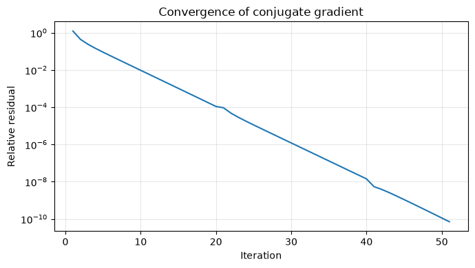
CG minimizes quadratic functions $\frac12x^\top Ax-b^\top x$ in a conjugated direction $A$ mutually relational functions. Stop checks are managed not by the number of iterations but by relative residual $\|b-Ax\|_2/\|b\|_2$.

Check with Python

residuals=[]
def cb(xk): residuals.append(np.linalg.norm(b-A_heat@xk)/np.linalg.norm(b))
x_cg,info=cg(A_heat,b,rtol=1e-10,callback=cb)
print("info:",info,"| iterations:",len(residuals),"| final relative residual:",f"{residuals[-1]:.2e}")
fig,ax=plt.subplots(figsize=(7,4)); ax.semilogy(range(1,len(residuals)+1),residuals)
ax.set_title("Convergence of conjugate gradient"); ax.set_xlabel("Iteration"); ax.set_ylabel("Relative residual")
ax.grid(True,which="both",alpha=.3); plt.tight_layout(); plt.show()

info: 0 | iterations: 51 | final relative residual: 7.13e-11

Reading the results

When the residual becomes monotonically small enough, info=0 shows convergence. However, small residuals do not directly guarantee the validity of the physical model. Boundary conditions, material constants, and mesh dependencies will be examined separately.

No.078: Pretreatment Method

Meaning in Practice

If the coefficient scale differs significantly, the number of iterations increases even with the same CG. Preprocessing is converted into an “easy-to-solve” form without changing the solution, and is timed for daily batch and control cycles.

Approach to Analysis and Modeling

Here, we use the Jacobi preprocessing $M^{-1}\approx A^{-1}$ that employs diagonal components. The more conditions you add, the faster the convergence generally becomes, but the total cost of creating and applying the preprocessing itself is used to determine the results.

Check with Python

scale=np.geomspace(1,1e3,n); D=sparse.diags(scale); A_scaled=D@A_heat@D; b_scaled=D@b
counts={}
for label,M in [("None",None),("Jacobi",LinearOperator((n,n),matvec=lambda x:x/A_scaled.diagonal()))]:
    hist=[]
    x,info=cg(A_scaled,b_scaled,rtol=1e-8,M=M,callback=lambda xk,h=hist:h.append(np.linalg.norm(b_scaled-A_scaled@xk)/np.linalg.norm(b_scaled)),maxiter=2000)
    counts[label]=(len(hist),hist[-1],info)
display(pd.DataFrame(counts,index=["iterations","final_residual","info"]).T)

	iterations	final_residual	info
None	1288.0	7.501723e-09	0.0
Jacobi	45.0	7.642589e-09	0.0

Reading the results

Jacobi preprocessing significantly reduces the number of iterations for issues worsened by diagonal scaling. For production, incomplete options like Cholesky are also considered, but we compare them by considering preprocessing build time, additional memory, and the number of reuses on multiple right-hand sides.

No.079: Sparse Matrix Solver

Meaning in Practice

Most matrices arising from local interactions are zero. By using sparse formats, you can handle finer meshes with the same computational resources without storing or calculating zeros.

Approach to Analysis and Modeling

$n\times n$ dense matrix generally requires about $8n^2$ bytes. The CSR format holds non-zero values, column numbers, and row pointers, and in this triple diagonal matrix, the number of non-zero numbers is limited to about $3n$. We also compare the solutions of the direct method spsolve and CG.

Check with Python

n_big=5000
A_big=sparse.diags([-np.ones(n_big-1),2.2*np.ones(n_big),-np.ones(n_big-1)],[-1,0,1],format="csr")
b_big=np.ones(n_big)
dense_mb=n_big*n_big*8/1024**2
sparse_mb=(A_big.data.nbytes+A_big.indices.nbytes+A_big.indptr.nbytes)/1024**2
t0=time.perf_counter(); x_direct=spsolve(A_big,b_big); elapsed=time.perf_counter()-t0
display(pd.DataFrame({"representation":["Dense (estimated)","CSR (actual)"],"memory_MB":[dense_mb,sparse_mb]}).round(3))
print("nonzeros:",A_big.nnz,"| spsolve time:",f"{elapsed:.4f}s","| relative residual:",f"{np.linalg.norm(b_big-A_big@x_direct)/np.linalg.norm(b_big):.2e}")

	representation	memory_MB
0	Dense (estimated)	190.735
1	CSR (actual)	0.191

nonzeros: 14998 | spsolve time: 0.0018s | relative residual: 1.27e-16

Reading the results

The actual memory of CSR is orders of magnitude smaller than the estimated value in dense format, and the residual is sufficiently small even with the direct method. However, even with sparse matrices, fill-in during decomposition increases memory, so direct or iterative methods are chosen depending on the size, structure, and number of right-hand sides of the matrix.

No.080: Large-Scale Matrix Computation

Meaning in Practice

In large-scale computing, it is more important to define only the necessary operations and return results within the budget of accuracy, time, and memory, rather than “creating a matrix.” It affects the frequency of updates to Digital Twins and production plans.

Approach to Analysis and Modeling

LinearOperator does not explicitly define the matrix and only defines $x\mapsto Ax$. A 1,000,000-dimensional triple diagonal action is performed using several vectors, where a dense matrix requires about 7.3 TiB. Performance evaluation should normally include warm-ups and repeated measurements, but here we examine structural differences.

Check with Python

n_matrix_free=1_000_000
def heat_matvec(x):
    y=2.2*x.copy(); y[1:]-=x[:-1]; y[:-1]-=x[1:]; return y
op=LinearOperator((n_matrix_free,n_matrix_free),matvec=heat_matvec,dtype=float)
x=np.ones(n_matrix_free); t0=time.perf_counter(); y=op@x; elapsed=time.perf_counter()-t0
dense_tib=n_matrix_free**2*8/1024**4
print(f"dimension: {n_matrix_free:,}")
print(f"dense matrix estimate: {dense_tib:,.1f} TiB")
print(f"matrix-free matvec: {elapsed:.4f}s | vector result memory: {y.nbytes/1024**2:.1f} MiB")
print("result sample:",y[:3],y[-3:])

dimension: 1,000,000
dense matrix estimate: 7.3 TiB
matrix-free matvec: 0.0026s | vector result memory: 7.6 MiB
result sample: [1.2 0.2 0.2] [0.2 0.2 1.2]

Reading the results

Even at 1,000,000 dimensions, you can perform matrix vector multiplication using regular memory as long as you only use the operational rules. Combining this with Krylov repetition avoids explicit generation of large matrices. However, in actual operation, performance design is required that includes communication between computing nodes, preprocessing, downtime conditions, and resumption design in case of failure.

Practical Implications Seen Through Target Exercise

Unevaluated cells for equipment × varieties can be converted into prototype priority using a low-rank structure. On the other hand, since prediction scores do not guarantee safety or machinability, exclusion from candidates due to hardware constraints and on-site testing are essential. On the computational side, by handling only the top-level components, subspaces, nonzero elements, and matrix vector products, the scale of problems can be increased.

In decision-making, not only model accuracy but also the following three aspects are managed simultaneously.

1. Business Value: How much can we reduce the number of prototypes, the startup period, and the waiting time for calculations?
2. numerical reliability: Whether verification error, residuals, convergence information, and reproducibility are being recorded
3. Safe Operation: Do not automatically approve recommendations, but pass equipment constraints and engineer reviews?

What is necessary for practical implementation

• Define conformity cross-departmentally, based on quality rates, CT, energy, and safety constraints.
• Auditing for random missing entries or selection biases where only successful cases are recorded
• Measuring performance under unknown conditions through time-series segmentation and verification that excludes entire equipment and varieties
• Record recommendation candidates, acceptance or rejection, and prototype results, then return to model renewal
• Load testing of sparse format, tolerance error, preprocessing, and time/memory limits at a production scale
• Manage models, data, seeds, libraries, and decision-makers in editions, and determine stopping conditions in case of abnormalities

Conclusion

In No.071–080, we identified manufacturing challenges ranging from recommending equipment candidates through low-rank matrix decomposition, to Krylov subspaces, eigenvalue approximation, CG, preprocessing, sparse matrices, and matrix-free calculations. A common principle is not to compute all the massive information but to select and calculate the structures necessary for decision-making. By separating mathematical approximation errors from on-site judgment risks, we advance from PoC to stable operation.

Consultations for Corporations

At Mathematical Laboratory, we support everything from problem organization to operational design, from test planning for equipment × varieties, recommendation and optimization models, accelerating CAE and large-scale sparse matrix calculations, to corporate training using field data.

📩 Contact Us: surikobo.co.jp/contact
Please feel free to consult us first.