Numerical Audit of Process Network Stability — 100 Exercises on Linear Algebra in Manufacturing No.051–No.060

When the effects between equipment are expressed in a matrix, “theoretically stable” alone is not sufficient for on-site judgment. In this paper, we use a hypothetical circular process consisting of four devices as the subject, treating everything from semi-constant matrix to matrix stability as a single audit procedure.

[!NOTE] This material is a notebook previously used by Surikoubo (or personally by the representative, Kazuyama), and has been reconstructed, edited, and published with the company’s permission.
All data listed is fictional and has no relation whatsoever to real companies, factories, or figures.

Introduction: Practical Challenges in Manufacturing Covered in This Article

Consider the line where load deviations from cutting, cleaning, heat treatment, and inspection carry over to the next shift. If we $\mathbf{x}_t$ state and $A$ propagation matrix, it becomes $\mathbf{x}_{t+1}=A\mathbf{x}_t+\boldsymbol{\varepsilon}_t$.

Common situations on site

• There are process-specific KPIs, but the ripple effects between processes are not being evaluated.
• There are simulation results, but sensitivity to parameter errors is unknown.
• Slow eigenvalue calculations on large-scale equipment data

Why is this issue so difficult to judge?

Stability is determined by the inherent structure of the entire matrix. In asymmetric matrices, even long-term stability can have short-term amplification, and measurement errors and rounding errors also affect judgment.

Overview of Exercise covered this time

Structural eigenvalues are evaluated in No.051 to 054, and numerical reliability is checked in No.055. Compare calculation methods in No.056–058, and integrate them into time response and stability judgment in No.059–060.

Preparing the Python environment

We use NumPy, pandas, Matplotlib, and SciPy. Fix the random number seed and separate the rounding of display and internal calculations.

import sys, numpy as np, pandas as pd, matplotlib, matplotlib.pyplot as plt
from scipy.linalg import expm
from scipy.sparse import diags
from scipy.sparse.linalg import eigsh
from IPython.display import display
rng=np.random.default_rng(51060)
np.set_printoptions(precision=4,suppress=True)
plt.rcParams.update({"figure.figsize":(7.2,4.2),"axes.grid":True})
print("Python",sys.version.split()[0],"NumPy",np.__version__,"pandas",pd.__version__,"Matplotlib",matplotlib.__version__)

Python 3.13.1 NumPy 2.5.1 pandas 3.0.3 Matplotlib 3.11.0

Creation of Fictional Data

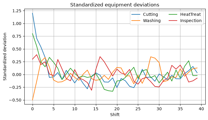
4. The impact on the next shift of the equipment is expressed by the nonnegative matrix $A$, generating 120 shifts. Diagonal components carry over themselves, while non-diagonal components carry over between processes. In practice, the estimated period and model version are recorded.

equipment=["Cutting","Washing","HeatTreat","Inspection"]
A=np.array([[.56,.10,.03,.02],[.08,.50,.11,.03],[.04,.09,.61,.10],[.03,.04,.12,.48]])
states=np.zeros((120,4)); states[0]=[1.2,-.5,.8,.3]
for t in range(1,120): states[t]=A@states[t-1]+rng.normal(0,.12,4)
display(pd.DataFrame(A,index=equipment,columns=equipment).round(2))
plt.plot(states[:40]); plt.title("Standardized equipment deviations"); plt.xlabel("Shift"); plt.ylabel("Standardized deviation"); plt.legend(equipment,ncol=2); plt.grid(True); plt.tight_layout(); plt.show()

	Cutting	Washing	HeatTreat	Inspection
Cutting	0.56	0.10	0.03	0.02
Washing	0.08	0.50	0.11	0.03
HeatTreat	0.04	0.09	0.61	0.10
Inspection	0.03	0.04	0.12	0.48

No.051: Semi-Constant Matrix

Meaning in Practice

It serves as the foundation to prevent unbalanced losses between processes and covariance matrices from returning negative evaluations. However, if there is a zero eigenvalue, there will be deviation directions that are not evaluated.

Approach to Analysis and Modeling

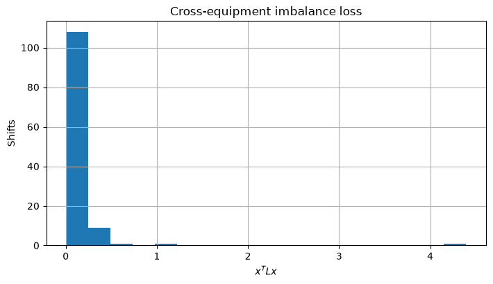
A symmetric matrix $Q$ satisfies $\mathbf{x}^TQ\mathbf{x}\ge0$ for any $\mathbf{x}$ if all eigenvalues are non-negative. We use Laplacian $L=D-W$ to penalize process discrepancies.

Check with Python

W=np.array([[0,1,.2,0],[1,0,.7,.1],[.2,.7,0,.9],[0,.1,.9,0]])
L=np.diag(W.sum(1))-W; ev=np.linalg.eigvalsh(L); loss=np.einsum("ij,jk,ik->i",states,L,states)
display(pd.DataFrame({"eigenvalue":ev}).round(6)); print("minimum loss",loss.min())
plt.hist(loss,bins=18); plt.title("Cross-equipment imbalance loss"); plt.xlabel(r"$x^T L x$"); plt.ylabel("Shifts"); plt.grid(True); plt.tight_layout(); plt.show()

	eigenvalue
0	-0.000000
1	0.725724
2	2.206091
3	2.868186

minimum loss 0.005229475856508912

Reading the results

Eigenvalues and losses are non-negative. Zero eigenvalues are a common mode where all equipment is identical but misaligned, so not only the KPIs for inter-process differences but also the overall center deviation KPIs are used together.

No.052: Rayleigh Commercial

Meaning in Practice

You can compare how likely candidate deviation patterns are to remain, and use it to prioritize improvement proposals.

Approach to Analysis and Modeling

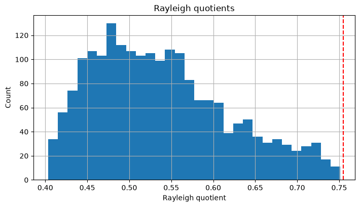
The $R(\mathbf{x})=\mathbf{x}^TS\mathbf{x}/\mathbf{x}^T\mathbf{x}$ for the symmetric part $S=(A+A^T)/2$ lies between the minimum and maximum eigenvalues.

Check with Python

S=(A+A.T)/2; X=rng.normal(size=(2000,4)); X/=np.linalg.norm(X,axis=1,keepdims=True)
rq=np.einsum("ij,jk,ik->i",X,S,X); sev=np.linalg.eigvalsh(S)
print("sample",rq.min(),rq.max(),"theory",sev[0],sev[-1])
plt.hist(rq,bins=30); plt.axvline(sev[-1],color="red",ls="--"); plt.title("Rayleigh quotients"); plt.xlabel("Rayleigh quotient"); plt.ylabel("Count"); plt.grid(True); plt.tight_layout(); plt.show()

sample 0.4034253637601614 0.7513199375074551 theory 0.3994312035852489 0.7546030144172374

Reading the results

Sample values are within the theoretical range. You can focus on monitoring process combinations close to the maximum values, but the long-term stability of asymmetric $A$ is checked separately with eigenvalues.

No.053: Gershgorin’s Theorem

Meaning in Practice

High-speed screening that estimates eigenvalue ranges from only the coefficient table, suitable for routine monitoring during model updates.

Approach to Analysis and Modeling

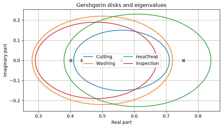
All eigenvalues are placed within a disk with a radius $r_i=\sum_{j\ne i}|a_{ij}|$ center $a_{ii}$ of each row. If the entire disk is within the unit circle, stability is sufficient.

Check with Python

c=np.diag(A); r=np.sum(abs(A),1)-abs(c); g=pd.DataFrame({"center":c,"radius":r,"right":c+r},index=equipment); display(g.round(3))
th=np.linspace(0,2*np.pi,300)
for name,ci,ri in zip(equipment,c,r): plt.plot(ci+ri*np.cos(th),ri*np.sin(th),label=name)
e=np.linalg.eigvals(A); plt.scatter(e.real,e.imag,c="black",marker="x"); plt.title("Gershgorin disks and eigenvalues"); plt.xlabel("Real part"); plt.ylabel("Imaginary part"); plt.legend(ncol=2); plt.grid(True); plt.tight_layout(); plt.show()

	center	radius	right
Cutting	0.56	0.15	0.71
Washing	0.50	0.22	0.72
HeatTreat	0.61	0.23	0.84
Inspection	0.48	0.19	0.67

Reading the results

Since the right edge of the entire disc is less than 1, stability can be guaranteed at a low cost. If the disk protrudes, it is not considered unstable and is then forwarded to precise eigenvalue calculation.

No.054: Perron-Frobenius Theorem

Meaning in Practice

Using a non-negative process matrix, we indicate the magnitude of common fluctuations and equipment configuration that remain over the long term, and determine the survey priority.

Approach to Analysis and Modeling

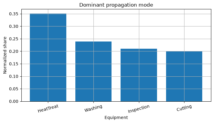
In positive matrices, spectral radius $\rho(A)$ is a positive simple eigenvalue, and the corresponding eigenvector has positive components. Normalize the sum to 1 and read the contribution.

Check with Python

vals,vecs=np.linalg.eig(A); ii=np.argmax(abs(vals)); rho=vals[ii].real; v=abs(vecs[:,ii].real); v/=v.sum()
pf=pd.DataFrame({"equipment":equipment,"share":v}).sort_values("share",ascending=False); display(pf.round(4)); print("spectral radius",rho)
plt.bar(pf.equipment,pf.share); plt.title("Dominant propagation mode"); plt.xlabel("Equipment"); plt.ylabel("Normalized share"); plt.xticks(rotation=15); plt.grid(True); plt.tight_layout(); plt.show()

	equipment	share
2	HeatTreat	0.3509
1	Washing	0.2395
3	Inspection	0.2104
0	Cutting	0.1993

spectral radius 0.754099720331183

Reading the results

The controlling eigenvalue is less than 1, indicating that heat treatment contributes significantly. This is not a determined cause or effect, but rather a priority for sensor scrutiny and improvement experiments.

No.055: Number of Conditions in a Matrix

Meaning in Practice

It shows how many times a small error in measurement or coefficient can be amplified into the result of the backward calculation of causal contribution.

Approach to Analysis and Modeling

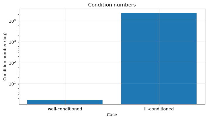
The number of 2-norm conditions is $\kappa_2(M)=\sigma_{max}/\sigma_{min}$. Compare good conditions with bad conditions where rows almost overlap.

Check with Python

Mg=np.array([[1,.2,.1],[.1,1.1,.2],[.2,.1,.9]]); Mb=np.array([[1,1.001,.1],[.5,.5004,.2],[.2,.2003,1]])
y=np.array([1,.7,.4]); d=np.array([1e-4,-1e-4,1e-4]); rows=[]
for name,M in [("well-conditioned",Mg),("ill-conditioned",Mb)]:
 z=np.linalg.solve(M,y); zp=np.linalg.solve(M,y+d); rows.append([name,np.linalg.cond(M),np.linalg.norm(zp-z)/np.linalg.norm(z)])
df=pd.DataFrame(rows,columns=["case","condition_number","relative_solution_change"]); display(df.round(6))
plt.bar(df.case,df.condition_number); plt.yscale("log"); plt.title("Condition numbers"); plt.xlabel("Case"); plt.ylabel("Condition number (log)"); plt.grid(True); plt.tight_layout(); plt.show()

	case	condition_number	relative_solution_change
0	well-conditioned	1.664609	0.000185
1	ill-conditioned	22771.393274	0.000957

Reading the results

In the negative condition matrix, contribution estimation is sensitive. Consider adding sensors, integrating variables, regularization, and limiting valid digits. The number of conditions is not the actual error but the ease of amplification in the worst-case scenario.

No.056: Power Multiplication

Meaning in Practice

Only the maximum eigenvalues and control modes are updated at low cost in large-scale models, and stability margins are regularly monitored.

Approach to Analysis and Modeling

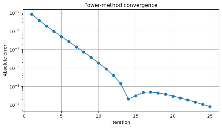
$\mathbf{v}_{k+1}=A\mathbf{v}_k/\|A\mathbf{v}_k\|$ iterates and estimates eigenvalues using the Rayleigh quotient. The convergence velocity depends on the ratio of eigenvalues.

Check with Python

v=np.ones(4)/2; hist=[]
for k in range(25):
 w=A@v; v=w/np.linalg.norm(w); hist.append(float(v@(A@v)/(v@v)))
df=pd.DataFrame({"iteration":range(1,26),"estimate":hist,"error":abs(np.array(hist)-rho)}); display(df.iloc[[0,1,2,4,9,24]].round(7))
plt.semilogy(df.iteration,df.error,marker="o"); plt.title("Power-method convergence"); plt.xlabel("Iteration"); plt.ylabel("Absolute error"); plt.grid(True); plt.tight_layout(); plt.show()

	iteration	estimate	error
0	1	0.745741	8.359300e-03
1	2	0.750208	3.892100e-03
2	3	0.752186	1.913300e-03
4	5	0.753591	5.087000e-04
9	10	0.754081	1.890000e-05
24	25	0.754100	1.000000e-07

Reading the results

The estimate converges to a governing eigenvalue. In the actual game, not only the number of repetitions but also the residual $\|A\mathbf{v}-\lambda\mathbf{v}\|$ is set as the stop condition.

No.057: Lanczos Method

Meaning in Practice

From the symmetric sparse matrix of many devices, only the edge eigenvalues are obtained with minimal memory, increasing the update frequency.

Approach to Analysis and Modeling

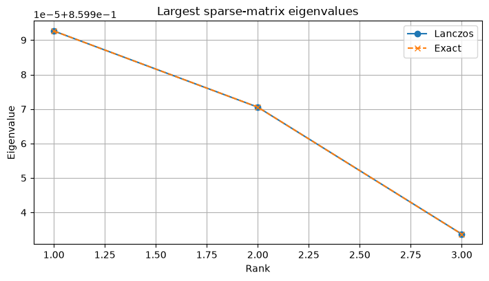
Projecting into the Krylov subspace to create triple diagonalization. Using eigsh, we find the top three eigenvalues of 400 facilities and compare them with known strict formulas.

Check with Python

n=400; LS=diags([.12*np.ones(n-1),.62*np.ones(n),.12*np.ones(n-1)],[-1,0,1],format="csr")
lv=eigsh(LS,k=3,which="LA",return_eigenvectors=False)[::-1]; exact=.62+.24*np.cos(np.arange(1,4)*np.pi/(n+1))
df=pd.DataFrame({"rank":[1,2,3],"Lanczos":lv,"exact":exact,"error":abs(lv-exact)}); display(df.round(10))
plt.plot(df["rank"],df.Lanczos,"o-",label="Lanczos"); plt.plot(df["rank"],df.exact,"x--",label="Exact"); plt.title("Largest sparse-matrix eigenvalues"); plt.xlabel("Rank"); plt.ylabel("Eigenvalue"); plt.legend(); plt.grid(True); plt.tight_layout(); plt.show()

	rank	Lanczos	exact	error
0	1	0.859993	0.859993	0.0
1	2	0.859971	0.859971	0.0
2	3	0.859934	0.859934	0.0

Reading the results

It does not convert to dense matrices and matches the exact value. For the asymmetric matrix, select the Arnoldi method and record the allowable error, maximum iteration, and residual.

No.058: QR Method

Meaning in Practice

You can inventory all eigenvalues and use them as a standard to verify partial iterative methods.

Approach to Analysis and Modeling

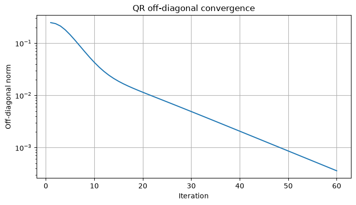
$A_k=Q_kR_k$, repeat $A_{k+1}=R_kQ_k$. Maintain eigenvalues in similarity transformations and converge diagonally in symmetric matrices.

Check with Python

Ak=S.copy(); off=[]
for k in range(60):
 Q,R=np.linalg.qr(Ak); Ak=R@Q; off.append(np.linalg.norm(Ak-np.diag(np.diag(Ak)),"fro"))
qv=np.sort(np.diag(Ak))[::-1]; tv=np.sort(np.linalg.eigvalsh(S))[::-1]; display(pd.DataFrame({"QR":qv,"library":tv,"error":abs(qv-tv)}).round(8))
plt.semilogy(range(1,61),off); plt.title("QR off-diagonal convergence"); plt.xlabel("Iteration"); plt.ylabel("Off-diagonal norm"); plt.grid(True); plt.tight_layout(); plt.show()

	QR	library	error
0	0.754603	0.754603	0.000000
1	0.560052	0.560052	0.000000
2	0.435912	0.435914	0.000002
3	0.399433	0.399431	0.000002

Reading the results

Even in a no-shift educational implementation, the library results will match. In production, we use faster and verified eigvalsh to avoid proprietary implementations.

No.059: Matrix Function

Meaning in Practice

From the temperature, concentration, and vibration models for continuous time, the state after any time and the return time are calculated.

Approach to Analysis and Modeling

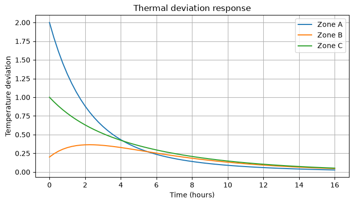
The solution to $\dot{\mathbf{x}}=F\mathbf{x}$ is $\mathbf{x}(t)=e^{Ft}\mathbf{x}(0)$. The matrix index is not an element-specific index.

Check with Python

F=np.array([[-.45,.16,0],[.08,-.34,.10],[0,.12,-.28]]); x0=np.array([2,.2,1]); tt=np.linspace(0,16,65); tr=np.array([expm(F*t)@x0 for t in tt])
print("eigenvalues",np.linalg.eigvals(F)); display(pd.DataFrame(tr[[0,16,32,64]],index=tt[[0,16,32,64]],columns=["Zone A","Zone B","Zone C"]).round(4))
plt.plot(tt,tr); plt.title("Thermal deviation response"); plt.xlabel("Time (hours)"); plt.ylabel("Temperature deviation"); plt.legend(["Zone A","Zone B","Zone C"]); plt.grid(True); plt.tight_layout(); plt.show()

eigenvalues [-0.5359+0.j -0.3573+0.j -0.1768+0.j]

	Zone A	Zone B	Zone C
0.0	2.0000	0.2000	1.0000
4.0	0.4321	0.3274	0.4242
8.0	0.1406	0.1839	0.2078
16.0	0.0275	0.0454	0.0518

Reading the results

The real part of eigenvalues is negative, and deviations are attenuated. Not only “stability,” but also the return time to the tolerance range is included in the conservation plan, and input, saturation, and delays are also separately verified.

No.060: Matrix Stability

Meaning in Practice

Integrate asymptotic stability, short-term maximum amplification, and stability margin to determine the criteria for alerts and re-identification.

Approach to Analysis and Modeling

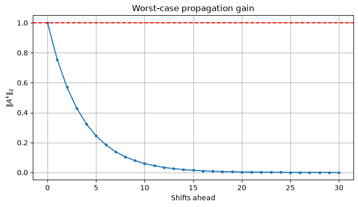
Discrete-time systems are asymptotic stable if $\rho(A)<1$. $\|A^k\|_2$ represents transient amplification in the worst direction. Set an internal threshold including estimated errors instead of boundary 1.

Check with Python

hh=np.arange(31); gain=np.array([np.linalg.norm(np.linalg.matrix_power(A,int(k)),2) for k in hh]); pi=int(np.argmax(gain))
display(pd.DataFrame({"metric":["spectral radius","margin","peak gain","peak shift"],"value":[rho,1-rho,gain[pi],pi]}).round(4))
plt.plot(hh,gain,marker="o",ms=3); plt.axhline(1,color="red",ls="--"); plt.title("Worst-case propagation gain"); plt.xlabel("Shifts ahead"); plt.ylabel(r"$\|A^k\|_2$"); plt.grid(True); plt.tight_layout(); plt.show()

	metric	value
0	spectral radius	0.7541
1	margin	0.2459
2	peak gain	1.0000
3	peak shift	0.0000

Reading the results

The model is asymptotic stable and does not show significant transient amplification. However, stress tests are performed on confidence intervals with coefficients, for example, $ho(A)\ge0.90$ is set as an internal trigger for re-identification.

Practical Implications Seen Through Target Exercise

This model is stable, but “less than 1” is not the only conclusion. There is a common mode invisible to semi-constant loss, and in the dominant mode, the contribution of heat treatment is large, and the number of conditions showed that the inverse calculation of causal contribution can become unstable. Simple boundaries, control value updates, large-scale partial calculations, and overall audits are used according to different applications.

What is necessary for practical implementation

1. Time synchronization, missed measurement handling, standardization, and unification of product types and equipment conditions
2. Testing prediction errors and residuals outside the learning period
3. Record the number of conditions, eigen-to-residuals, allowable errors, and library versions
4. Aligning stability margins, transitional peaks, and return times with quality and maintenance standards
5. Determine drift detection, relearning conditions, approvers, and rollbacks

Mathematical stability is not about safety or quality assurance itself. Combine FMEA, control charts, equipment knowledge, and experimental planning.

Conclusion

No.051–060 connect matrix structure, eigenvalue boundaries, dominance modes, numerical sensitivity, calculation methods, and time response to a consistent stability audit. What matters is clearly stating what is guaranteed under which assumptions and under what conditions it is reevaluated.

Consultations for Corporations

At the Suriku Kobo, we support everything from organizing equipment and quality data to process propagation models, anomaly sign monitoring, simulation, site explanations, and operational design.

📩 Contact Us: surikobo.co.jp/contact
Please feel free to consult us first.