Manufacturing Decision-Making Connected by Linear Algebra—10 Practical Questions on Equipment Design, Maintenance, Quality, and Management

This article deals with the No.091〜No.100 of 100 linear algebra exercises in connection with decision-making in a fictional precision parts factory. From Finite Element Method (FEM) to digital twins, manufacturing DI, and generative AI, we will examine the common structure behind seemingly different technologies—representing states with vectors and relationships and transformations with matrices—using executable Python code.

[!NOTE] This material is a notebook previously used by Surikoubo (or personally by the representative, Kazuyama), and has been reconstructed, edited, and published with the company’s permission.
All data listed is fictional and has no relation whatsoever to real companies, factories, or figures.

Introduction: Practical Challenges in Manufacturing Covered in This Article

On the manufacturing floor, equipment deformation, allocation planning, transition of failure states, search for similar products, and demand fluctuations are often handled by separate departments. However, these can be discussed on the same computational basis by representing states as vectors and interactions as matrices. The purpose of this article is not to memorize formulas, but to help you judge Which quantities are defined as states and which relationships are made into matrices?.

Common situations on site

• The design department has analysis results, but the connection with production conditions is weak.
• Production plans are adjusted using spreadsheets, and constraints and objective functions are implicitly implemented
• Sensor data is accumulated, but cannot be fully utilized for estimating equipment status or searching for similar cases.
• The causal relationship between management indicators and on-site KPIs is fragmented by department.

Why is this issue so difficult to judge?

Observations contain noise, conditions are not directly visible, and multiple constraints and evaluation axes compete. Also, what can be calculated mathematically is not the same as what can be adopted in the field. You need to design the model that includes units, data granularity, constraints, update frequency, and accountability.

Overview of Exercise covered this time

No.	Theme	Questions in the Manufacturing Industry
091	FEM	Is jig displacement under load within an acceptable range?
092	optimization problem	How to allocate limited facility time
093	Markov chain	How will the equipment condition evolve in the future?
094	Linear Algebra in Quantum Mechanics	How to read states, operators, and expected values
095	Recommendation System	How to present candidate process conditions
096	Vector Search	How to find similar past troubles
097	Simulation	How much is the risk of shortages due to uncertain demand?
098	Digital twin	How to update virtual equipment based on actual measurements
099	Manufacturing DI	How to Summarize Business Sentiment from Multiple KPIs
100	Why linear algebra is important in the AI era	How to oversee AI input/output

Preparing the Python environment

Vector and matrix calculations are performed in NumPy, table formats are checked in pandas, optimization is performed in SciPy, and visualization is done in matplotlib. The random number generator is fixed so that rerunning it yields the same result.

import sys
import numpy as np
import pandas as pd
import matplotlib
import matplotlib.pyplot as plt
from scipy.optimize import linprog

try:
    import japanize_matplotlib  # Enable Japanese display
except ImportError:
    pass

np.set_printoptions(precision=3, suppress=True)
pd.set_option("display.precision", 3)
rng = np.random.default_rng(20250701)

print(f"Python: {sys.version.split()[0]}")
print(f"NumPy: {np.__version__}, pandas: {pd.__version__}, matplotlib: {matplotlib.__version__}")

Python: 3.13.1
NumPy: 2.5.1, pandas: 3.0.3, matplotlib: 3.11.0

Creation of Fictional Data

The target is a fictional precision parts factory that processes products A through D. It generates daily demand, temperature, spindle vibration, machining errors, and power consumption. We embed a weak relationship where increased demand and rising temperatures affect equipment load, but this is not the actual value for real companies.

n_days = 120
day = np.arange(n_days)
temperature = 23 + 5*np.sin(2*np.pi*day/30) + rng.normal(0, 0.8, n_days)
demand = 205 + 0.28*day + 18*np.sin(2*np.pi*day/14) + rng.normal(0, 10, n_days)
vibration = 1.8 + 0.006*day + 0.035*(temperature-23) + rng.normal(0, 0.10, n_days)
machining_error = 5.0 + 0.85*vibration + 0.05*(temperature-23) + rng.normal(0, 0.25, n_days)
power = 115 + 0.16*demand + 2.2*vibration + rng.normal(0, 2.5, n_days)

factory = pd.DataFrame({
    "day": day + 1, "demand_units": demand.round(0), "temperature_C": temperature,
    "vibration_mm_s": vibration, "error_um": machining_error, "power_kWh": power
})
print(factory.head().to_string(index=False))
print("\nKey Statistics")
print(factory.drop(columns="day").describe().loc[["mean", "std", "min", "max"]].round(2))

 day  demand_units  temperature_C  vibration_mm_s  error_um  power_kWh
   1         204.0         23.124           1.870     7.056    156.019
   2         211.0         24.208           1.742     6.626    154.307
   3         208.0         24.933           1.873     6.896    152.340
   4         217.0         25.779           1.889     6.629    156.710
   5         228.0         27.362           2.080     6.781    158.471

Key Statistics
      demand_units  temperature_C  vibration_mm_s  error_um  power_kWh
mean        220.88          23.06            2.14      6.80     155.25
std          19.36           3.64            0.25      0.37       4.31
min         163.00          16.76            1.61      5.89     141.74
max         263.00          29.13            2.63      7.67     164.78

fig, axes = plt.subplots(2, 1, figsize=(10, 6), sharex=True)
axes[0].plot(factory["day"], factory["demand_units"], color="tab:blue")
axes[0].set(title="Daily demand for fictitious factories", ylabel="Needs (number/Day)")
axes[0].grid(True, alpha=0.3)
axes[1].plot(factory["day"], factory["vibration_mm_s"], color="tab:red")
axes[1].set(title="Trends in Equipment Vibration", xlabel="days", ylabel="Vibration (mm/s）")
axes[1].grid(True, alpha=0.3)
plt.tight_layout()
plt.show()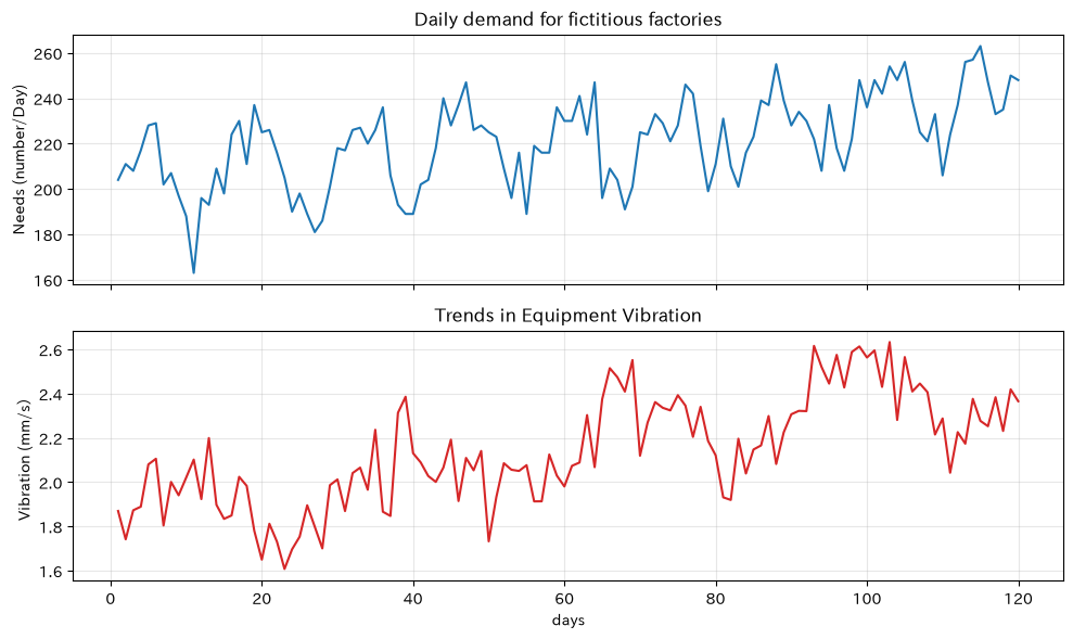

No.091: FEM — Evaluating Jig Displacement as a System of Equations

Meaning in Practice

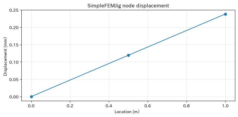
When jigs or frames deform under load, it affects machining accuracy and tool life. In the Finite Element Method (FEM), the continuum is divided into smaller elements, and deformation is calculated using node displacement as an unknown. Here, we simplify to one-dimensional spring elements and check the computational framework.

Approach to Analysis and Modeling

The basic formula of a static linear FEM is

$$\mathbf{K}\mathbf{u}=\mathbf{f}$$

That’s right. $\mathbf{K}$ is the stiffness matrix, $\mathbf{u}$ is the node displacement, and $\mathbf{f}$ is the external force. Assemble the element stiffness $k=EA/L$ into the entire matrix and solve it except for the degrees of freedom at the fixed end. In practice, the validity of material nonlinearity, contact, temperature, and boundary conditions is also verified.

Check with Python

E, area, length = 210e9, 4.0e-4, 0.50  # Pa, m^2, m
k = E * area / length
K = k * np.array([[1, -1, 0], [-1, 2, -1], [0, -1, 1]], dtype=float)
force = np.array([0, 0, 20_000.0])
u = np.zeros(3)
u[1:] = np.linalg.solve(K[1:, 1:], force[1:])
fem_result = pd.DataFrame({"node": [0, 1, 2], "location_m": [0, .5, 1.0], "displacement_mm": u*1e3})
print(fem_result.to_string(index=False))

plt.figure(figsize=(8, 4))
plt.plot(fem_result["location_m"], fem_result["displacement_mm"], marker="o")
plt.title("SimpleFEMJig node displacement")
plt.xlabel("Location (m）"); plt.ylabel("Displacement (mm）"); plt.grid(True, alpha=.3); plt.tight_layout(); plt.show()

 Nodal Position _m Displacement _mm
  0   0.0  0.000
  1   0.5  0.119
  2   1.0  0.238

Reading the results

The displacement increases toward the free end, with a maximum displacement of about 0.24 mm. If the allowable value is 0.10 mm, design changes are necessary. However, meshing the mesh alone does not guarantee accuracy; design reviews confirm whether fixing conditions, load direction, and material constants match the actual product.

No.092: Optimization Problem—Turning Facility Time into Profit

Meaning in Practice

When you can’t complete all orders, instead of handling the high-volume projects, you set production quantities by clearly stating profit, equipment time, and demand limits.

Approach to Analysis and Modeling

If the quantity by product is $\mathbf{x}$, marginal profit is $\mathbf{c}$, equipment utilization coefficient is $\mathbf{A}$, and capacity is $\mathbf{b}$,

\mathrm{s.t.}\quad \mathbf{A}\mathbf{x}\leq\mathbf{b},\;\mathbf{x}\geq0$$ This is the linear plan. Coefficients are agreed upon by both accounting and the site side, and arrangements, lots, and delivery dates are added as integer constraints as needed. ### Check with Python ```python products = np.array(["ProductsA", "ProductsB", "ProductsC", "ProductsD"]) profit = np.array([42, 55, 38, 70]) # 100 yen per piece A = np.array([[1.2, 1.8, 1.0, 2.4], [0.8, 0.6, 1.5, 1.2]]) capacity = np.array([520, 360]) demand_max = np.array([180, 140, 160, 100]) opt = linprog(-profit, A_ub=A, b_ub=capacity, bounds=list(zip(np.zeros(4), demand_max)), method="highs") plan = pd.DataFrame({"Products": products, "Production Quantity": opt.x, "Requirement ceiling": demand_max, "marginal_interest_value_100_yen": profit, "value_value_100_yen": opt.x*profit}) print(plan.round(1).to_string(index=False)) print(f"\nTotal Marginal Profit: {-opt.fun:,.0f} value_100_yen") print("Equipment usage / ability:", np.round(A @ opt.x, 1), "/", capacity) ``` Product Production Quantity Demand Upper Limit Marginal Profit _100 yen Profit Contribution _ 100 yen Product A 180.0 180 42 7560.0 Product B 114.3 140 55 6285.7 Product C 98.3 160 38 3734.9 Product D 0.0 100 70 0.0 Total Marginal Profit: 17,581 100 yen Equipment usage / capacity: [520. 360.] / [520 360] ### Reading the results The optimal solution allocates capacity to higher-value products and allows you to check which equipment has reached its limit. Decimal solutions are standard plans, and in practice, after rounding them into lots, they are re-evaluated for any constraint violations. Sensitivity analysis with a ±10% change in profit coefficient is also effective for confirming the robustness of the plan. ## No.093: Markov Chains—Predicting Future Distribution of Equipment Conditions ### Meaning in Practice By understanding how equipment transitions between "normal, caution, and failure," it becomes possible to plan maintenance personnel and spare parts based on future failure probabilities, rather than responding after a shutdown. ### Approach to Analysis and Modeling Each row of the transition matrix $\mathbf{P}$ represents the current state, each column represents the next-day state, and the sum of rows is 1. The state probability $\boldsymbol{\pi}_t$ is $\boldsymbol{\pi}_{t+1}=\boldsymbol{\pi}_t\mathbf{P}$ will be updated. We also check whether the assumption of ignoring history dependencies is too strong. ### Check with Python ```python states = ["normal", "Note", "malfunction"] P = np.array([[.92, .075, .005], [.25, .65, .10], [.55, .30, .15]]) pi = np.array([1., 0., 0.]) history = [pi.copy()] for _ in range(30): pi = pi @ P history.append(pi.copy()) markov = pd.DataFrame(history, columns=states) print(markov.iloc[[0, 1, 7, 14, 30]].round(3)) plt.figure(figsize=(8, 4)) for s in states: plt.plot(markov.index, markov[s], label=s) plt.title("Trends in equipment condition probability"); plt.xlabel("elapsed date"); plt.ylabel("State probability") plt.grid(True, alpha=.3); plt.legend(); plt.tight_layout(); plt.show() ``` Normal Attention Fault 0 1.000 0.000 0.000 1 0.920 0.075 0.005 7 0.790 0.184 0.026 14 0.782 0.191 0.027 30 0.782 0.191 0.027 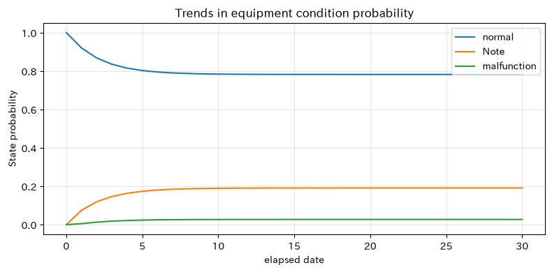 ### Reading the results Even if you start from normal, the probability of attention and malfunction accumulates over time and approaches a certain distribution. The probability of failure on day 30 is not 'the probability of breaking down even once within 30 days,' but rather **30Probability of being out of state at the time of the day**. It is important not to confuse this difference with conservation KPIs. ## No.094: Linear Algebra in Quantum Mechanics—Understanding State, Operator, and Expected Value ### Meaning in Practice This is not about immediately introducing quantum computing into factories. In quantum mechanics, states are represented as complex vectors and observational surveys as matrices, making this a condensed teaching material that encapsulates the meaning of linear algebra. It also serves as a basic vocabulary in technical evaluations such as quantum sensing and materials calculations. ### Approach to Analysis and Modeling For normalized state $|\psi\rangle$, observations are represented by Hermitian matrices $\mathbf{H}$. The expected value is $\langle H\rangle=\langle\psi|\mathbf{H}|\psi\rangle$ is here. The eigenvalue is the candidate measurement result, and the probability is the absolute square of the projection to the eigenvector. ### Check with Python ```python psi = np.array([np.sqrt(.7), np.exp(1j*np.pi/4)*np.sqrt(.3)]) H = np.array([[1.0, 0.2-0.1j], [0.2+0.1j, 2.0]]) eigenvalues, eigenvectors = np.linalg.eigh(H) probabilities = np.abs(eigenvectors.conj().T @ psi)**2 expected = np.vdot(psi, H @ psi).real quantum = pd.DataFrame({"Measured value (eigenvalue)": eigenvalues, "measurement probability": probabilities}) print(quantum.round(4).to_string(index=False)) print(f"Probability sum: {probabilities.sum():.4f}, expected value: {expected:.4f}") ``` Measurement value (eigenvalue) Measurement probability 0.952 0.505 2.048 0.495 Sum of probabilities: 1.0000, Expected value: 1.4944 ### Reading the results The sum of the measurement probabilities equals 1, and the expected value matches the probability-weighted mean of the eigenvalue. Even with the advent of complex numbers, the structure of decision-making is "state× transformation× evaluation." In technology selection, rather than promoting quantum superiority, the target problem, errors, and comparison conditions with classical calculations are clearly indicated. ## No.095: Recommendation System — Supplementing Candidate Process Conditions ### Meaning in Practice If the combination of varieties and processing conditions increases, it becomes impossible to test everything. Candidates with untested conditions are presented from past evaluation queues, narrowing down the scope of exploration for skilled participants. ### Approach to Analysis and Modeling Approximate the evaluation matrix $\mathbf{R}$ of breed × conditions with the low-rank matrix $\mathbf{U}_k\mathbf{\Sigma}_k\mathbf{V}_k^{\mathsf T}$. This is a simple educational case that supplements missing values, and in production, it deals with losses from observed elements alone, bias, time series partitioning, and safety constraints. ### Check with Python ```python R = np.array([[92, 88, np.nan, 70], [85, np.nan, 80, 65], [60, 68, 90, np.nan], [np.nan, 72, 94, 88], [78, 82, np.nan, 74]], float) row_mean = np.nanmean(R, axis=1, keepdims=True) filled = np.where(np.isnan(R), row_mean, R) U, s, Vt = np.linalg.svd(filled, full_matrices=False) pred = (U[:, :2] * s[:2]) @ Vt[:2] rows, cols = np.where(np.isnan(R)) recommendations = pd.DataFrame({"variety": [f"variety{i+1}" for i in rows], "Untested conditions": [f"condition{j+1}" for j in cols], "Predictive Evaluation": pred[rows, cols]}) print(recommendations.sort_values("Predictive Evaluation", ascending=False).round(1).to_string(index=False)) ``` Variety Untested Conditions Predictive Evaluation Variety 1 Condition 3 82.3 Variety 5 Condition 3 81.4 Variety 4 Condition 1 79.5 Variety 2 Condition 2 78.9 Variety 3 Condition 4 76.4 ### Reading the results You can prioritize untested conditions with high predictive ratings. However, the recommended values are not quality assurance but rather the order of additional tests. It is necessary to exclude conditions that do not meet safety or standards in advance, and to return the measured results after adoption back into the queue. ## No.096: Vector Search—Searching for Similar Past Troubles ### Meaning in Practice Even if the expression of trouble records differs for each person in charge, by converting vibration, temperature, power, errors, and other factors into common vectors, you can search for past cases close to the current situation. ### Approach to Analysis and Modeling For vector $\mathbf{x},\mathbf{y}$ standardized with scale differences, cosine similarity $\cos\theta=\mathbf{x}^{\mathsf T}\mathbf{y}/(\|\mathbf{x}\|_2\|\mathbf{y}\|_2)$ is used. Standardization conditions, feature weights, and the definition of correct answers in search results all determine performance. ### Check with Python ```python features = factory[["temperature_C", "vibration_mm_s", "error_um", "power_kWh"]] Z = (features - features.mean()) / features.std(ddof=0) query = Z.iloc[-1].to_numpy() past = Z.iloc[:-1].to_numpy() similarity = past @ query / (np.linalg.norm(past, axis=1)*np.linalg.norm(query)) top = np.argsort(similarity)[-5:][::-1] search_result = factory.iloc[top][["day", "temperature_C", "vibration_mm_s", "error_um", "power_kWh"]].copy() search_result["cosine_similarity"] = similarity[top] print("Search Targets: 120day") print(search_result.round(3).to_string(index=False)) ``` Search Target: Day 120 day temperature_C vibration_mm_s error_um power_kWh cosine_similarity 114 18.442 2.376 6.683 164.381 0.950 91 22.531 2.322 6.633 157.342 0.878 87 20.357 2.299 6.824 159.235 0.873 77 23.134 2.204 6.860 163.935 0.838 115 17.441 2.277 6.833 162.336 0.823 ### Reading the results The highest-ranking similarity date serves as the entry point for investigating cases close to the current state. Even if the values are close, the causes may not be the same. Replacement parts, alarms, and work records are recorded together, and maintenance personnel's evaluations are fed back into search quality. ## No.097: Simulation — Comparing Inventory Policies under Demand Fluctuations ### Meaning in Practice If you decide safety stock based solely on average demand, you overlook stockouts during periods of high volatility. Generate numerous demand scenarios and compare the relationship between service levels and inventory levels. ### Approach to Analysis and Modeling Generate correlated multi-variety demand with $\mathbf{d}=\boldsymbol{\mu}+\mathbf{L}\mathbf{z}$. $\mathbf{L}$ is the Cholesky factor of the covariance matrix. Ignoring correlation can lead to underestimating the risks of simultaneous stockouts or capacity concentration. ### Check with Python ```python mu = np.array([210, 150, 120]) cov = np.array([[625, 180, 90], [180, 400, 120], [90, 120, 225]]) L = np.linalg.cholesky(cov) sim_demand = mu + rng.standard_normal((10000, 3)) @ L.T safety_levels = np.array([0.0, 0.5, 1.0, 1.5, 2.0]) rows = [] std = np.sqrt(np.diag(cov)) for z in safety_levels: stock = mu + z*std fill_rate = np.minimum(sim_demand, stock).sum() / sim_demand.sum() all_filled = np.mean(np.all(sim_demand <= stock, axis=1)) rows.append((z, stock.sum(), fill_rate, all_filled)) policy = pd.DataFrame(rows, columns=["safety factor", "total inventory", "quantity adequacy rate", "Simultaneous Adequacy Rate of All Varieties"]) print(policy.round(3).to_string(index=False)) plt.figure(figsize=(8, 4)) plt.plot(policy["total inventory"], policy["quantity adequacy rate"], marker="o", label="quantity adequacy rate") plt.plot(policy["total inventory"], policy["Simultaneous Adequacy Rate of All Varieties"], marker="s", label="Simultaneous Adequacy Rate of All Varieties") plt.title("The trade-off between inventory and service levels"); plt.xlabel("Total Inventory (units)"); plt.ylabel("Service level") plt.grid(True, alpha=.3); plt.legend(); plt.tight_layout(); plt.show() ``` Safety factor, total inventory, quantity fulfillment rate, simultaneous fulfillment rate of all varieties 0.0 480.0 0.949 0.207 0.5 510.0 0.975 0.407 1.0 540.0 0.989 0.642 1.5 570.0 0.996 0.826 2.0 600.0 0.999 0.933 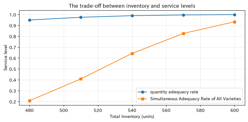 ### Reading the results The more inventory you build, the higher the fulfillment rate, but the incremental effect gradually diminishes. Also, even if the quantity fulfillment rate is high, the probability of meeting all varieties simultaneously is relatively low. In management meetings, we first define which service levels will be protected as contracts and customer value. ## No.098: Digital Twin—Updating Virtual Facilities with Measured Values ### Meaning in Practice Digital twins are not limited to 3D displays. This system continuously corrects predictions based on physical models through sensor observations to estimate the invisible state of equipment. ### Approach to Analysis and Modeling State $\mathbf{x}_t$ is predicted using the transition matrix $\mathbf{F}$, and the residual is calculated from observation $\mathbf{y}_t$ and observation matrix $\mathbf{H}$. Here, we update the steady Kalman filter type. $\hat{\mathbf{x}}\leftarrow\hat{\mathbf{x}}+\mathbf{K}(\mathbf{y}-\mathbf{H}\hat{\mathbf{x}})$ simplified implementation. ### Check with Python ```python observed = factory[["vibration_mm_s", "temperature_C"]].to_numpy() F = np.array([[1.0, 0.002], [0.0, 1.0]]) H = np.eye(2) gain = np.diag([0.35, 0.55]) x = observed[0].copy() estimated = [] for y in observed: x_pred = F @ x x = x_pred + gain @ (y - H @ x_pred) estimated.append(x.copy()) estimated = np.array(estimated) plt.figure(figsize=(9, 4)) plt.plot(factory["day"], observed[:, 0], alpha=.45, label="Measured vibration") plt.plot(factory["day"], estimated[:, 0], linewidth=2, label="Twin estimation") plt.title("Updating the digital twin status based on actual measurements"); plt.xlabel("days"); plt.ylabel("Vibration (mm/s）") plt.grid(True, alpha=.3); plt.legend(); plt.tight_layout(); plt.show() print(f"Measured vibration on the final day={observed[-1,0]:.3f}, estimated vibration={estimated[-1,0]:.3f} mm/s") ``` 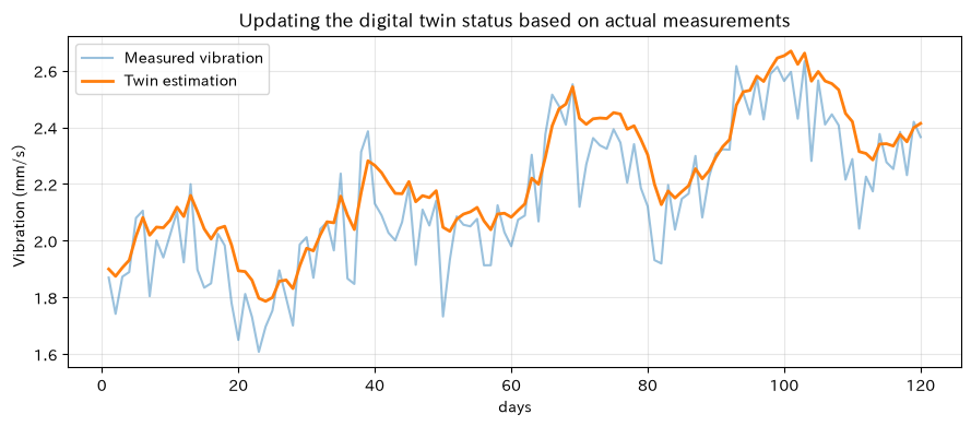 Final day measured vibration = 2.366, estimated vibration = 2.414 mm/s ### Reading the results Estimates follow changes while smoothing out measured noise. The greater the gain, the more sensitive it is to actual measurements; the smaller the gain, the more emphasis is placed on physical models. In production, operational design includes sensor calibration, communication failures, model update responsibilities, and fail-safe in case of abnormalities. ## No.099: Manufacturing DI—Extracting Common Changes from Multiple KPIs ### Meaning in Practice The Manufacturing DI (Diffusion Index) is an indicator that summarizes the spread of improvement, stagnation, and deterioration. Here, we combine the standardization of on-site KPIs with key components to confirm common directions for order receipt, operation, quality, and inventory. ### Approach to Analysis and Modeling Response-based DI is generally defined as "improvement rate minus deterioration rate." On the other hand, continuous KPIs can eigendely decompose the covariance matrix of the normalized matrix $\mathbf{Z}$ and use the first eigenvector as the weight of the common factor. Since the sign is arbitrary, align so that the order increase is positive. ### Check with Python ```python months = pd.date_range("2025-01-01", periods=12, freq="MS") latent = np.linspace(-1.2, 1.1, 12) + rng.normal(0, .25, 12) kpi = pd.DataFrame({ "Order received": 100 + 12*latent + rng.normal(0, 3, 12), "utilization_rate": 78 + 5*latent + rng.normal(0, 1.5, 12), "Yield Rate": 96 + .7*latent + rng.normal(0, .25, 12), "inventory turnover": 7 + .8*latent + rng.normal(0, .3, 12), }, index=months) Z = (kpi-kpi.mean())/kpi.std(ddof=0) eigval, eigvec = np.linalg.eigh(np.cov(Z, rowvar=False, ddof=0)) weights = eigvec[:, -1] if weights[0] < 0: weights *= -1 di = Z @ weights / np.linalg.norm(weights) print(pd.DataFrame({"KPI": kpi.columns, "DIWeight": weights}).round(3).to_string(index=False)) print(f"No.1Explanation rate of principal components: {eigval[-1]/eigval.sum():.1%}") plt.figure(figsize=(9, 4)) plt.plot(months, di, marker="o"); plt.axhline(0, color="black", linewidth=.8) plt.title("Manufacturing of fictitious factoriesDI(Standardized Index)"); plt.xlabel("month"); plt.ylabel("DI") plt.grid(True, alpha=.3); plt.tight_layout(); plt.show() ``` Weight on KPI DI Orders 0.518 Utilization rate: 0.507 Yield Rate: 0.490 Inventory turnover: 0.485 Explanation rate of the first principal component: 88.9% 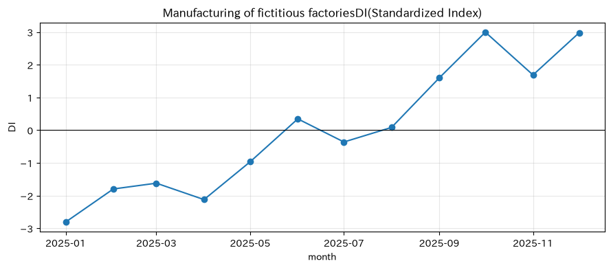 ### Reading the results A positive DI indicates a common phase where multiple KPIs are above average, while a negative one indicates a weak phase. If the explanatory rate is low, summarizing a single index is risky. Since reestimating weights monthly changes the meaning of the indicators, the base period and revised rules are fixed, and the original KPI is also recorded. ## No.100: Why Linear Algebra Matters in the AI Era—Overseeing Embedding and Attention ### Meaning in Practice Generative AI converts manuals, anomaly records, drawing attributes, and more into vectors, searching for and integrating related information. When users understand linear algebra, they can verify AI behaviors such as similarity, weight, dimension, and normalization. ### Approach to Analysis and Modeling Attention converts the dot product of query $\mathbf{Q}$ and key $\mathbf{K}$ into weights in softmax, and weights the value $\mathbf{V}$. $$\operatorname{Attention}(Q,K,V)=\operatorname{softmax}\left(\frac{QK^{\mathsf T}}{\sqrt{d}}\right)V$$ Weights provide clues for explanation, but they do not guarantee causal basis or correctness. ### Check with Python ```python labels = ["spindle vibration", "coolant temperature", "processing error", "Tool usage time"] K_ai = np.array([[.9,.1,.2], [.1,.9,.2], [.7,.2,.6], [.5,.1,.8]]) V_ai = np.array([[.8,.2], [.2,.4], [.9,.7], [.6,.9]]) # Amount of information on anomalies and conservation Q_ai = np.array([[.8,.1,.7]]) # "Causes of Reduced Machining Accuracy" scores = Q_ai @ K_ai.T / np.sqrt(K_ai.shape[1]) attention = np.exp(scores-scores.max()) attention /= attention.sum(axis=1, keepdims=True) context = attention @ V_ai ai_result = pd.DataFrame({"Sources": labels, "Attentionweight": attention.ravel()}) print(ai_result.sort_values("Attentionweight", ascending=False).round(3).to_string(index=False)) print("Integration context [abnormal, preserve] =", context.round(3)) plt.figure(figsize=(8, 4)) plt.bar(labels, attention.ravel(), color="tab:purple") plt.title("Regarding inquiriesAttentionweight"); plt.xlabel("Sources"); plt.ylabel("weight") plt.grid(True, axis="y", alpha=.3); plt.tight_layout(); plt.show() ``` Source: Attention Weight Processing error 0.279 Tool usage time 0.274 Spindle vibration 0.259 Coolant Temperature 0.187 Integration context [Anomalous, Safeguard] = [[0.661 0.569]] 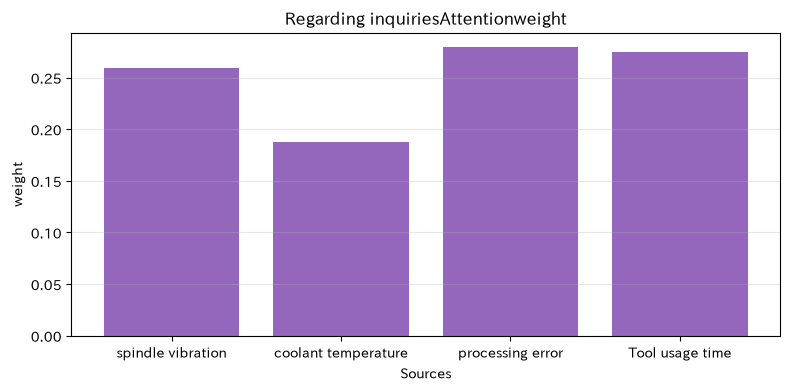 ### Reading the results The larger the product of the inquiry vector, the higher the weight of the information source, and the value vector is strongly reflected in the response. AI implementation involves managing the version of the searched document, access rights, source indication, human approval, and recording incorrect answers. Linear algebra is not only for making your own model, but also for **AIA common language for overseeing output**. ## Practical Implications Seen Through Target Exercise What all 10 problems have in common is the process of converting reality into vectors, relationships into matrices, and then converting them into outputs tailored to the objective. 1. **State definition comes first, algorithm comes later.**: What is considered a single state, row, or column determines the outcome. 2. **Managing Units and Metrics**: It is important not to haphazardly mix rigidity, demand, vibration, and writing features. 3. **Clearly state constraints and uncertainties**: Instead of treating the optimal solution or predicted value as a final value, it indicates the acceptable range and sensitivity. 4. **Preparing the materials for judgment without replacing human judgment**: Recommendations, searches, DI, and AI are tools that narrow down candidates to be verified. ## What is necessary for practical implementation - Linking management issues with KPIs and determining the tolerance for errors - Standardize data definition, credits, missing data, sensor calibration, and version management - Separate learning and validation periods and agree on comparative metrics with current methods - Checking operational load and exception handling in small-scale PoCs including field personnel - Define model owners, approvers, update frequency, downtime conditions, and audit logs - Evaluate effectiveness not only by accuracy but also by stopping time, yield, inventory, and decision time ## Conclusion FEM, optimization, state transitions, recommendation, search, simulation, digital twins, DI, and AI are all connected by a common foundation called linear algebra. What matters is not memorizing difficult formulas, but correctly translating states, relationships, objectives, and constraints into matrices and vectors, and returning the results to real-world judgment. This notebook is a small reproduction example, so please verify it step-by-step using actual data and operational constraints during implementation. ## Consultations for Corporations At Mathematical Laboratory, we support you according to the maturity of your challenges, covering everything from organizing manufacturing data, mathematical model design, PoC, on-site implementation, to training. You can consult from the early stages, such as "We have data but can't determine a theme" or "We want to connect analysis results to decision-making." > 📩 **Contact Us**: [surikobo.co.jp/contact](https://surikobo.co.jp/contact) > Please feel free to consult us first.