Matrix Factorization for Connecting Missing Multi-Product Quality Data to Decision-Making — 100 Exercises on Linear Algebra in Manufacturing No.061–No.070

In manufacturing sites, equipment conditions, inspection characteristics, product types, and time zones combine to quickly create a large quality datasheet. In this article, we use a fictional precision parts factory as a subject to examine Solving simultaneous equations stably, compressing quality variations into a few factors, and supplementing missing test values in ways that lead to on-site decision-making.

The goal is not to memorize the method name. (1) What you want to calculate quickly and stably, (2) How much information can be compressed, (3) Under what conditions should missing values be compensated, and you can choose the decomposition that best fits your purpose. The data is fictional generated in Python and does not depend on external data.

[!NOTE] This material is a notebook previously used by Surikoubo (or personally by the representative, Kazuyama), and has been reconstructed, edited, and published with the company’s permission.
All data listed is fictional and has no relation whatsoever to real companies, factories, or figures.

Introduction: Practical Challenges in Manufacturing Covered in This Article

Consider a factory that processes 12 types with 8 machines, inspecting six characteristics: dimensions, roundness, roughness, hardness, vibration, and temperature. It is not possible to measure all combinations every time, and the measurement matrix may be incomplete. Additionally, the characteristics correlate with each other through common factors such as processing load and thermal effects.

What is needed in this situation is not simply to calculate the average value, but to solve calibration calculations stably, extract the main causes of variation, and estimate unmeasured values while managing compression errors. Matrix decomposition serves as a common language for breaking large computations into meaningful smaller ones.

Common situations on site

• Using the same coefficient matrix, different measurements are solved multiple times for each day
• Inspection characteristics increase, and it’s unclear which metrics should be prioritized in meetings.
• I want to visualize multi-variety data, but I can’t compare it in 6D.
• Defects occur due to omission of inspection or communication disconnection, and simple average completion eliminates variation between varieties.
• Although the compression model is highly accurate, the site cannot explain the latent factors.

Why is this issue so difficult to judge?

There are multiple options for matrix decomposition, each with different premises and purposes. Cholesky decomposition is strong for symmetric positive definite matrices, QR decomposition is stable at least squares, and SVD excels at ranking and information diagnosis but requires a large computational load. PCA describes centralized fluctuations, while NMF describes non-negative additive patterns. In defect compensation, even if there is a low-rank characteristic, if the defect is biased toward a specific variety, estimation is dangerous.

Overview of Exercise covered this time

No.	Theme	Judgment in the manufacturing industry
061	LU Decomposition	Can multiple calibration calculations be streamlined with the same equipment model?
062	Cholesky Decomposition	Can covariance and normal equations be solved with a small computational complexity?
063	QR Decomposition	Can Proofreading Regression Including Multicollinearity Be Solved Reliably?
064	SVD	What are the independent variation directions and effective ranks of the quality matrix?
065	Low-rank approximation	How much information can be stored with a few factors?
066	PCA	Can varieties be compared based on key quality fluctuation axes?
067	NMF	Can non-negative non-negative contributions be divided into additive causal patterns?
068	Tensor Breakdown	Can compression be maintained while maintaining the three-way structure × characteristics of the variety× equipment,
069	CUR decomposition	Can approximation be explained using actual representative varieties and characteristics?
070	matrix completion	How far can unmeasured values be compensated from low-rank structures?

Preparing the Python environment

Perform matrix calculations with NumPy, tables with pandas, and visualization with Matplotlib. Avoid relying on SciPy or machine learning libraries, and make the breakdown a short implementation that allows you to track the contents. Fix the seed of the random number generator and separate the rounding of the display from the accuracy of internal calculations.

import sys
import numpy as np
import pandas as pd
import matplotlib
import matplotlib.pyplot as plt
from IPython.display import display

np.set_printoptions(precision=4, suppress=True)
rng = np.random.default_rng(20260712)
print(f"Python {sys.version.split()[0]} / NumPy {np.__version__} / pandas {pd.__version__} / Matplotlib {matplotlib.__version__}")

Python 3.13.1 / NumPy 2.5.1 / pandas 3.0.3 / Matplotlib 3.11.0

Creation of Fictional Data

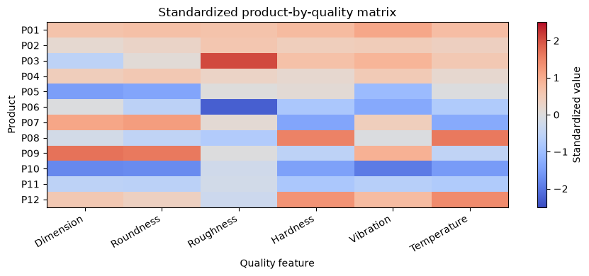
We produce tensors with 12 varieties, 8 equipment, and 6 inspection characteristics. Behind them are three latent factors: ‘processing load,’ ‘thermal effect,’ and ‘surface condition,’ and the observed values are set to include small measurement noise. The quality matrix $X$ for analysis is a table of variety× characteristics averaging equipment directions, and each column is standardized.

products = [f"P{i:02d}" for i in range(1, 13)]
machines = [f"M{i:02d}" for i in range(1, 9)]
features = ["Dimension", "Roundness", "Roughness", "Hardness", "Vibration", "Temperature"]

product_factor = rng.normal(size=(12, 3))
machine_factor = rng.normal(scale=0.45, size=(8, 3))
feature_loading = np.array([[0.90, 0.15, 0.10], [0.75, 0.10, 0.30],
                            [0.15, 0.05, 0.95], [0.05, 0.90, 0.10],
                            [0.55, 0.25, 0.45], [0.10, 0.95, 0.05]])
quality_tensor = np.einsum("pr,fr->pf", product_factor, feature_loading)[:, None, :] + np.einsum("mr,fr->mf", machine_factor, feature_loading)[None, :, :]
quality_tensor += rng.normal(scale=0.10, size=quality_tensor.shape)
raw_matrix = quality_tensor.mean(axis=1)
X = (raw_matrix - raw_matrix.mean(axis=0)) / raw_matrix.std(axis=0, ddof=1)
quality_df = pd.DataFrame(X, index=products, columns=features)
display(quality_df.round(2))

fig, ax = plt.subplots(figsize=(9, 4))
im = ax.imshow(X, cmap="coolwarm", aspect="auto", vmin=-2.5, vmax=2.5)
ax.set_title("Standardized product-by-quality matrix")
ax.set_xlabel("Quality feature"); ax.set_ylabel("Product")
ax.set_xticks(range(len(features)), features, rotation=30, ha="right")
ax.set_yticks(range(len(products)), products); ax.grid(False)
fig.colorbar(im, ax=ax, label="Standardized value"); fig.tight_layout(); plt.show()

	Dimension	Roundness	Roughness	Hardness	Vibration	Temperature
P01	0.64	0.70	0.64	0.78	1.07	0.72
P02	0.17	0.29	0.57	0.42	0.47	0.39
P03	-0.54	0.09	2.07	0.67	0.87	0.53
P04	0.44	0.54	0.31	0.19	0.49	0.19
P05	-1.49	-1.41	0.02	0.11	-1.05	-0.03
P06	-0.03	-0.56	-2.27	-0.81	-1.34	-0.73
P07	1.08	1.21	0.13	-1.40	0.43	-1.33
P08	-0.18	-0.51	-0.72	1.52	-0.05	1.61
P09	1.70	1.62	-0.02	-0.55	0.93	-0.50
P10	-1.79	-1.75	-0.24	-1.45	-1.94	-1.53
P11	-0.53	-0.58	-0.20	-0.81	-0.63	-0.74
P12	0.54	0.36	-0.30	1.32	0.75	1.41

No.061: LU Decomposition

Meaning in Practice

When solving calibration coefficients and process balance as $mathbf{A}mathbf{x}=mathbf{b}$, the $A$ representing the equipment structure may be the same, but only the daily observation $b$ may change. Once LU decomposition, you can efficiently solve multiple cases using forward and backward assignments.

Approach to Analysis and Modeling

Divide the matrix into lower triangle matrix $L$ and upper triangle matrix $U$ into $A=LU$, and solve in the order of $Lmathbf{y}=mathbf{b}$ and $Umathbf{x}=mathbf{y}$. In general-purpose practical implementations, row exchange $PA=LU$ is necessary to avoid destabilization caused by zero or too small pivots. Here, to make the principle easier to understand, we use a prime diagonal example that does not require row swapping.

Check with Python

def lu_decompose(A):
    A = A.astype(float); n = len(A); L = np.eye(n); U = np.zeros_like(A)
    for i in range(n):
        U[i, i:] = A[i, i:] - L[i, :i] @ U[:i, i:]
        if abs(U[i, i]) < 1e-12: raise ValueError("Pivoting is required")
        L[i+1:, i] = (A[i+1:, i] - L[i+1:, :i] @ U[:i, i]) / U[i, i]
    return L, U

A_cal = np.array([[4., 1., 0.5], [1., 3., 0.4], [0.5, 0.4, 2.5]])
B_cal = np.array([[12., 10.], [8., 9.], [6., 7.]])  # two operating days
L, U = lu_decompose(A_cal)
Y = np.linalg.solve(L, B_cal); coef_lu = np.linalg.solve(U, Y)
display(pd.DataFrame(L).round(3)); display(pd.DataFrame(U).round(3))
display(pd.DataFrame(coef_lu, index=["Feed", "Speed", "Cooling"], columns=["Day A", "Day B"]).round(3))
print(f"reconstruction error = {np.linalg.norm(A_cal - L @ U):.2e}")
print(f"maximum residual = {np.max(np.abs(A_cal @ coef_lu - B_cal)):.2e}")

	0	1	2
0	1.000	0.0	0.0
1	0.250	1.0	0.0
2	0.125	0.1	1.0

	0	1	2
0	4.0	1.00	0.500
1	0.0	2.75	0.275
2	0.0	0.00	2.410

	Day A	Day B
Feed	2.379	1.697
Speed	1.652	2.152
Cooling	1.660	2.116

reconstruction error = 0.00e+00
maximum residual = 1.78e-15

Reading the results

The reconstruction error and residual are at the rounding error level, and the right side for two days was solved simultaneously from the same decomposition. It is suitable for daily calibration that reuses coefficient matrices. However, in actual operation, instead of custom functions, a verified library with pivot selection is used, and the number of conditions is also monitored.

No.062: Cholesky Decomposition

Meaning in Practice

Covariance matrices of quality characteristics and regularized coefficient matrices of least squares tend to be symmetric positive definites, and using Cholesky decomposition allows solving with less computational complexity and memory than general decomposition.

Approach to Analysis and Modeling

The symmetric positive definite matrix $A$ can be uniquely decomposed with $A=LL^{\mathsf T}$. A positive definite is a property that is $z^{\mathsf T}Az>0$ for any nonzero $z$. Symmetry alone is not enough; we must check whether the minimum eigenvalue is correct.

Check with Python

cov = np.cov(X, rowvar=False) + 0.05 * np.eye(X.shape[1])
chol = np.linalg.cholesky(cov)
target = np.ones(len(features))
weights = np.linalg.solve(chol.T, np.linalg.solve(chol, target))
weights /= target @ weights
chol_table = pd.DataFrame({"Feature": features, "Portfolio weight": weights})
display(chol_table.round(3))
print(f"minimum eigenvalue = {np.linalg.eigvalsh(cov).min():.4f}")
print(f"factorization error = {np.linalg.norm(cov - chol @ chol.T):.2e}")

	Feature	Portfolio weight
0	Dimension	0.791
1	Roundness	0.171
2	Roughness	0.653
3	Hardness	0.244
4	Vibration	-1.139
5	Temperature	0.280

minimum eigenvalue = 0.0507
factorization error = 3.85e-16

Reading the results

Since the minimum eigenvalue is positive and the decomposition error is sufficiently small, it satisfies the assumption that it is a positive definite value. The weights here are examples of synthetic quality indicators that consider correlations, but whether negative weights are permissible in business operations is a separate constraint. We distinguish between what can be solved numerically and what is reasonable as a KPI.

No.063: QR Decomposition

Meaning in Practice

When estimating dimensional deviations from strongly correlated explanatory variables such as temperature, speed, and load, the normal equation tends to amplify errors. QR decomposition directly decomposes the design matrix and solves calibration regression relatively stably.

Approach to Analysis and Modeling

$D=QR$ is $Q^{\mathsf T}Q=I$, and $R$ is the upper triangle. The least squares problem $\min_\beta\|D\beta-y\|_2$ is replaced by $R\beta=Q^{\mathsf T}y$. Since the canonical equation $D^{\mathsf T}D$ almost squares the number of conditions, QR is a choice stronger against rounding errors.

Check with Python

n = 80
temperature = rng.normal(180, 4, n)
load = 0.85 * temperature + rng.normal(0, 2, n)
speed = rng.normal(1200, 60, n)
D = np.column_stack([np.ones(n), temperature - 180, load - load.mean(), (speed - 1200) / 100])
y = 0.20 + 0.035 * D[:, 1] - 0.020 * D[:, 2] + 0.08 * D[:, 3] + rng.normal(0, 0.08, n)
Q, R = np.linalg.qr(D, mode="reduced")
beta_qr = np.linalg.solve(R, Q.T @ y)
beta_lstsq = np.linalg.lstsq(D, y, rcond=None)[0]
display(pd.DataFrame({"Term": ["Intercept", "Temperature", "Load", "Speed/100"], "QR": beta_qr, "lstsq": beta_lstsq}).round(4))
print(f"orthogonality error = {np.linalg.norm(Q.T @ Q - np.eye(Q.shape[1])):.2e}")
print(f"condition(D)={np.linalg.cond(D):.1f}, condition(D.T@D)={np.linalg.cond(D.T @ D):.1f}")

	Term	QR	lstsq
0	Intercept	0.1934	0.1934
1	Temperature	0.0334	0.0334
2	Load	-0.0203	-0.0203
3	Speed/100	0.0829	0.0829

orthogonality error = 6.77e-16
condition(D)=8.9, condition(D.T@D)=78.4

Reading the results

The least squares solutions of QR and NumPy coincide. Since the number of conditions for a normal equation is greater than the design matrix, we understand why we do not explicitly create a normal equation under strongly correlated conditions. However, interpreting coefficients requires separate experimental planning and confounding management.

No.064: SVD (Singular Value Decomposition)

Meaning in Practice

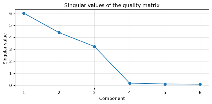
SVD divides the quality matrix into “variety-side patterns,” “importance,” and “characteristic patterns.” By observing the attenuation of singular values, you can diagnose how many independent factors actually move the six characteristics.

Approach to Analysis and Modeling

Any $m\times n$ matrix can be decomposed with $X=U\Sigma V^{\mathsf T}$. The singular value $\sigma_i$ is non-negative and arranged in descending order, and its square represents the energy of each component. Small singular values indicate noise direction and redundancy, but important minor fluctuations in the process should not be automatically considered unnecessary.

Check with Python

U, s, Vt = np.linalg.svd(X, full_matrices=False)
sv_df = pd.DataFrame({"Component": np.arange(1, len(s)+1), "Singular value": s, "Energy ratio": s**2 / np.sum(s**2)})
display(sv_df.round(4))
fig, ax = plt.subplots(figsize=(7, 3.5))
ax.plot(sv_df["Component"], sv_df["Singular value"], marker="o")
ax.set_title("Singular values of the quality matrix")
ax.set_xlabel("Component"); ax.set_ylabel("Singular value")
ax.grid(True, alpha=0.3); fig.tight_layout(); plt.show()
print(f"reconstruction error = {np.linalg.norm(X - U @ np.diag(s) @ Vt):.2e}")

	Component	Singular value	Energy ratio
0	1	6.0129	0.5478
1	2	4.3933	0.2924
2	3	3.2389	0.1589
3	4	0.1811	0.0005
4	5	0.1097	0.0002
5	6	0.0889	0.0001

reconstruction error = 1.07e-14

Reading the results

Singularities rapidly decrease from the top and reflect a small number of latent factors set at the time of generation. SVD serves as the benchmark for ranking assessments. The number of retained components is determined not only by bending but also by factors such as reconstruction error, anomaly detection sensitivity, and explainability.

No.065: Low-Rank Approximation

Meaning in Practice

With quality dashboards and edge terminals, you may not retain all data as is, but rather approximate only the main factors. Low-rank approximation quantifies the trade-off between information volume and storage/computation costs.

Approach to Analysis and Modeling

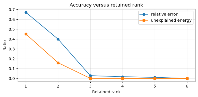
The $X_k=U_k\Sigma_kV_k^{\mathsf T}$, which leaves only the upper $k$ components of SVD, minimizes Frobenius norm error within the rank $k$ matrix. Compare the relative error and cumulative contribution rate, and select a $k$ acceptable for business purposes.

Check with Python

records = []
for k in range(1, len(s)+1):
    Xk = U[:, :k] @ np.diag(s[:k]) @ Vt[:k]
    records.append([k, np.linalg.norm(X-Xk)/np.linalg.norm(X), np.sum(s[:k]**2)/np.sum(s**2)])
rank_df = pd.DataFrame(records, columns=["Rank", "Relative error", "Cumulative energy"])
display(rank_df.round(4))
fig, ax = plt.subplots(figsize=(7, 3.5))
ax.plot(rank_df["Rank"], rank_df["Relative error"], marker="o", label="relative error")
ax.plot(rank_df["Rank"], 1-rank_df["Cumulative energy"], marker="s", label="unexplained energy")
ax.set_title("Accuracy versus retained rank")
ax.set_xlabel("Retained rank"); ax.set_ylabel("Ratio")
ax.grid(True, alpha=0.3); ax.legend(); fig.tight_layout(); plt.show()

	Rank	Relative error	Cumulative energy
0	1	0.6725	0.5478
1	2	0.3997	0.8403
2	3	0.0283	0.9992
3	4	0.0174	0.9997
4	5	0.0109	0.9999
5	6	0.0000	1.0000

Reading the results

The higher your rank, the less error becomes monotonous, but the improvement gradually narrows. Even if a small number of components can retain most variation, local phenomena such as specification deviations may appear on the residual side. It is necessary to design not only the compression ratio but also the residual management chart.

No.066: PCA (Principal Component Analysis)

Meaning in Practice

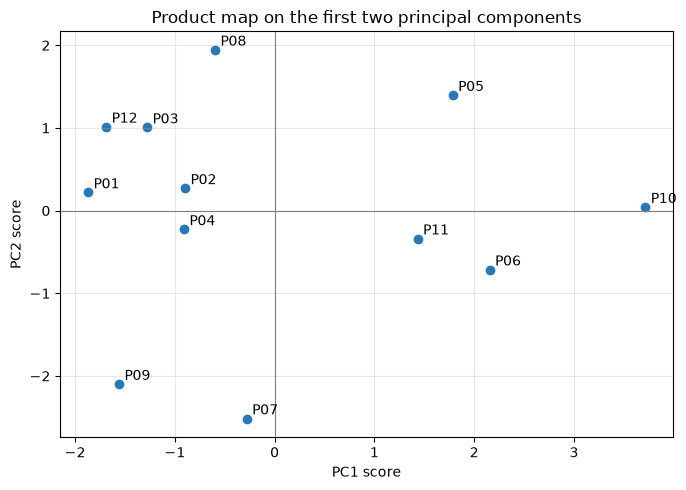
PCA consolidates correlated quality characteristics into a few synthetic axes and compares similar variations or off-topic varieties in two dimensions. This serves as the gateway to visualizing “which varieties are comprehensively different” during quality meetings.

Approach to Analysis and Modeling

From the SVD of the centralized matrix $X$, we get a score $Z=U\Sigma=XV$ and a load $V$. Standardized PCAs exclude unit differences, but they do not necessarily equal the importance of process capability or tolerances. Since the signs are invertible, interpret them in relative orientation.

Check with Python

scores = U[:, :2] * s[:2]
loadings = Vt[:2].T
display(pd.DataFrame(loadings, index=features, columns=["PC1", "PC2"]).round(3))
fig, ax = plt.subplots(figsize=(7, 5))
ax.scatter(scores[:, 0], scores[:, 1], color="#2878B5")
for i, name in enumerate(products): ax.annotate(name, scores[i], xytext=(4, 3), textcoords="offset points")
ax.axhline(0, color="gray", linewidth=0.8); ax.axvline(0, color="gray", linewidth=0.8)
ax.set_title("Product map on the first two principal components")
ax.set_xlabel("PC1 score"); ax.set_ylabel("PC2 score")
ax.grid(True, alpha=0.3); fig.tight_layout(); plt.show()

	PC1	PC2
Dimension	-0.413	-0.440
Roundness	-0.452	-0.430
Roughness	-0.270	0.105
Hardness	-0.355	0.561
Vibration	-0.543	-0.083
Temperature	-0.362	0.537

Reading the results

Similar varieties share six characteristic fluctuation patterns. From the load capacity, you can check whether each shaft is closer to dimensions and roundness, or closer to hardness and temperature. Varieties that are distant are candidates for investigation, but do not defectively; instead, stratify differences in variety specifications before identifying the cause.

No.067: NMF (Non-Negative Matrix Factorization)

Meaning in Practice

For non-negative data such as defect count or contribution, NMF, which combines non-negative cause patterns, may be easier to explain than PCA, where positive and negative factors cancel each other out. You can read “How many defective modes are included in each variety.”

Approach to Analysis and Modeling

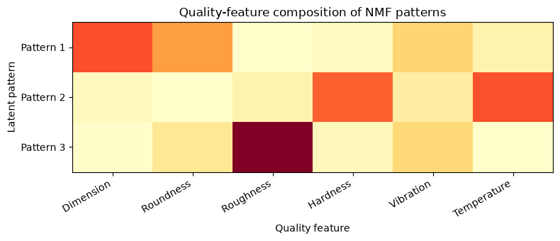
$D\approx WH$ and impose $D,W,H\ge0$. Here, we use the multiplicative update to reduce Frobenius errors. The solution depends on the initial value or scale and is not unique. Check the stability of multiple seeds and consistency with field labels.

Check with Python

D_defect = np.maximum(raw_matrix - raw_matrix.min(axis=0) + 0.15, 0)
k_nmf = 3
W = rng.random((D_defect.shape[0], k_nmf)) + 0.1
H = rng.random((k_nmf, D_defect.shape[1])) + 0.1
eps = 1e-10
for _ in range(800):
    H *= (W.T @ D_defect) / (W.T @ W @ H + eps)
    W *= (D_defect @ H.T) / (W @ H @ H.T + eps)
H_scaled = H / H.sum(axis=1, keepdims=True)
display(pd.DataFrame(H_scaled, index=["Pattern 1", "Pattern 2", "Pattern 3"], columns=features).round(3))
print(f"relative NMF error = {np.linalg.norm(D_defect-W@H)/np.linalg.norm(D_defect):.3f}")
fig, ax = plt.subplots(figsize=(8, 3.5))
ax.imshow(H_scaled, cmap="YlOrRd", aspect="auto")
ax.set_title("Quality-feature composition of NMF patterns")
ax.set_xlabel("Quality feature"); ax.set_ylabel("Latent pattern")
ax.set_xticks(range(len(features)), features, rotation=30, ha="right")
ax.set_yticks(range(3), ["Pattern 1", "Pattern 2", "Pattern 3"]); ax.grid(False)
fig.tight_layout(); plt.show()

	Dimension	Roundness	Roughness	Hardness	Vibration	Temperature
Pattern 1	0.426	0.302	0.002	0.025	0.182	0.063
Pattern 2	0.028	0.003	0.063	0.404	0.081	0.421
Pattern 3	0.009	0.108	0.684	0.033	0.165	0.001

relative NMF error = 0.036

Reading the results

Each pattern can be read as a non-negative characteristic construction, making it easier to replace causal hypotheses with field terminology. However, latent patterns are statistical co-occurrences and do not prove physical causes. You can reproduce the initial values by changing them, or verify them with maintenance history or experiments.

No.068: Tensor Decomposition

Meaning in Practice

If you × the characteristics of the product × equipment into a matrix, the pattern that appeared in the equipment is lost. Tensor decomposition maintains a three-way structure, simultaneously compressing varieties, equipment, and characteristics.

Approach to Analysis and Modeling

Here, we use HOSVD to project the matrix expanded into each mode into SVD and project onto the upper basis. $T\approx G\times_1U_p\times_2U_m\times_3U_f$ is represented by the core tensor $G$ and the factor matrix $U_p,U_m,U_f$. Rank $(r_p,r_m,r_f)$ is selected for each axis.

Check with Python

T = quality_tensor
Up = np.linalg.svd(T.reshape(T.shape[0], -1), full_matrices=False)[0][:, :3]
Um = np.linalg.svd(T.transpose(1,0,2).reshape(T.shape[1], -1), full_matrices=False)[0][:, :2]
Uf = np.linalg.svd(T.transpose(2,0,1).reshape(T.shape[2], -1), full_matrices=False)[0][:, :3]
core = np.einsum("pa,mb,fc,pmf->abc", Up, Um, Uf, T)
T_hat = np.einsum("pa,mb,fc,abc->pmf", Up, Um, Uf, core)
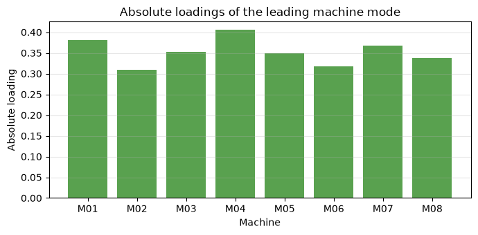
machine_loading = pd.DataFrame(Um, index=machines, columns=["Machine mode 1", "Machine mode 2"])
display(machine_loading.round(3))
print(f"original shape={T.shape}, core shape={core.shape}")
print(f"relative HOSVD error = {np.linalg.norm(T-T_hat)/np.linalg.norm(T):.3f}")
fig, ax = plt.subplots(figsize=(7, 3.5))
ax.bar(machines, np.abs(Um[:, 0]), color="#59A14F")
ax.set_title("Absolute loadings of the leading machine mode")
ax.set_xlabel("Machine"); ax.set_ylabel("Absolute loading")
ax.grid(True, axis="y", alpha=0.3); fig.tight_layout(); plt.show()

	Machine mode 1	Machine mode 2
M01	-0.381	0.148
M02	-0.309	-0.463
M03	-0.352	-0.144
M04	-0.405	0.709
M05	-0.349	-0.034
M06	-0.318	-0.425
M07	-0.368	0.158
M08	-0.337	-0.182

original shape=(12, 8, 6), core shape=(3, 2, 3)
relative HOSVD error = 0.308

Reading the results

We were able to compress the original 12×8×6 data into 3×2×3 cores and a three-factor matrix. Equipment with a high absolute value of equipment mode is a candidate contributing to common variation. However, since the signs and rotations are arbitrary, they are not directly due to “equipment defects,” so residuals are checked for each piece of equipment.

No.069: CUR Decomposition

Meaning in Practice

The latent vectors of SVD are a mixture of multiple characteristics and can be difficult to explain. CUR decomposition can be described as an approximation using “representative characteristics” and “representative varieties,” selecting the actual columns $C$ and row $R$ in the source data.

Approach to Analysis and Modeling

$X\approx CUR$ is used, and the importance of columns and rows is determined by the leverage score of the higher-level singular vector. Here, prioritize reproducibility and decisively select the top scores, with the central matrix set as $U=C^+XR^+$. While representativeness can be achieved, it is necessary to check that the columns are not biased toward homogeneous ones.

Check with Python

k_cur, n_cols, n_rows = 2, 3, 5
col_score = np.sum(Vt[:k_cur]**2, axis=0)
row_score = np.sum(U[:, :k_cur]**2, axis=1)
col_idx = np.argsort(col_score)[-n_cols:]
row_idx = np.argsort(row_score)[-n_rows:]
C_cur, R_cur = X[:, col_idx], X[row_idx, :]
U_cur = np.linalg.pinv(C_cur) @ X @ np.linalg.pinv(R_cur)
X_cur = C_cur @ U_cur @ R_cur
display(pd.DataFrame({"Selected feature": np.array(features)[col_idx], "Leverage score": col_score[col_idx]}).round(3))
display(pd.DataFrame({"Selected product": np.array(products)[row_idx], "Leverage score": row_score[row_idx]}).round(3))
print(f"relative CUR error = {np.linalg.norm(X-X_cur)/np.linalg.norm(X):.3f}")

	Selected feature	Leverage score
0	Roundness	0.39
1	Temperature	0.42
2	Hardness	0.44

	Selected product	Leverage score
0	P05	0.189
1	P08	0.206
2	P09	0.295
3	P07	0.330
4	P10	0.382

relative CUR error = 0.241

Reading the results

The selected columns and rows represent real characteristics and varieties that best represent the latent axis. While it is easy to use for site presentations and representative sample design, if there are fewer options, the error is greater than the optimal low-rank approximation of SVD. It clearly states the exchange conditions for representativeness and accuracy.

No.070: Matrix and Row Completion

Meaning in Practice

If you can compensate for the missing values caused by skipping inspections or temporary sensor stoppages, monitoring can continue. However, the complementary values are model estimates, not observations, and do not automatically replace shipment determination.

Approach to Analysis and Modeling

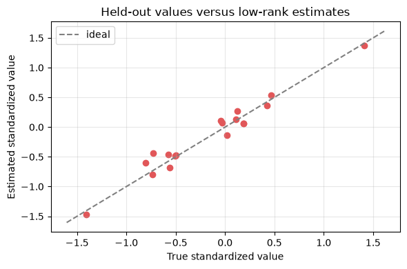
Low-rank matrices are calculated while minimizing errors on the observation set $\Omega$. Here, we use a simple Soft-Impute procedure to fix observations and iteratively update missing values using rank 3 SVD approximations. Evaluation measures RMSE using artificial validation defects that are not used for learning.

Check with Python

mask_observed = rng.random(X.shape) > 0.22
# Ensures that observations remain in each row and column
mask_observed[:, 0] = True; mask_observed[0, :] = True
X_missing = X.copy(); X_missing[~mask_observed] = np.nan
col_mean = np.nanmean(X_missing, axis=0)
X_fill = np.where(mask_observed, X_missing, col_mean)
for _ in range(150):
    u_i, s_i, vt_i = np.linalg.svd(X_fill, full_matrices=False)
    low_rank = u_i[:, :3] @ np.diag(s_i[:3]) @ vt_i[:3]
    updated = np.where(mask_observed, X, low_rank)
    if np.linalg.norm(updated-X_fill) < 1e-7: break
    X_fill = updated
missing_rmse = np.sqrt(np.mean((X_fill[~mask_observed]-X[~mask_observed])**2))
mean_fill = np.where(mask_observed, X, col_mean)
baseline_rmse = np.sqrt(np.mean((mean_fill[~mask_observed]-X[~mask_observed])**2))
print(f"missing cells = {(~mask_observed).sum()} / {X.size}")
print(f"low-rank completion RMSE = {missing_rmse:.3f}")
print(f"column-mean baseline RMSE = {baseline_rmse:.3f}")
fig, ax = plt.subplots(figsize=(6, 4))
ax.scatter(X[~mask_observed], X_fill[~mask_observed], color="#E15759")
lims = [X[~mask_observed].min()-.2, X[~mask_observed].max()+.2]
ax.plot(lims, lims, "--", color="gray", label="ideal")
ax.set_title("Held-out values versus low-rank estimates")
ax.set_xlabel("True standardized value"); ax.set_ylabel("Estimated standardized value")
ax.grid(True, alpha=0.3); ax.legend(); fig.tight_layout(); plt.show()

missing cells = 18 / 72
low-rank completion RMSE = 0.126
column-mean baseline RMSE = 0.767

Reading the results

In artificially hidden cells, you can directly compare the RMSE of low-rank completion and column average. For data with common factors like this, it is worthwhile to use a low-rank structure. However, if the chip only occurs during the actual breakdown, the loss is not random, and the verification results become more optimistic. Flags and uncertainties are assigned to complementary values, and critical tests are remeasured.

Practical Implications Seen Through Target Exercise

Matrix decomposition is not a one-size-fits-all method; it is a toolbox tailored to specific purposes.

• solve an equation: If you want to reuse coefficient matrices, choose LU; for symmetric positive definites, choose Cholesky; for least squares, choose QR as a candidate.
• Understanding the structure: Diagnose effective rank with SVD and manage accuracy and cost with low-rank approximation.
• explain: Use PCA for centralized variations, NMF for non-negative additive contributions, and CUR if you need a real representative matrix
• Maintain multidirectionality: Do not easily flatten the characteristics × the type × equipment; consider tensor disassembly
• Dealing with defects: Make assumptions of matrix completion, validation missing, baseline comparison, and estimation flags mandatory

What is necessary for practical implementation

1. Defining Objectives and Losses: Clarify the primary objectives of compression, visualization, prediction, and gap compensation.
2. Unify data granularity: Align variety, equipment, time, measurement units, and standard change history
3. Monitor the assumptions: Check the mechanisms of symmetry, positive fixability, number of conditions, rank, non-negativity, and defect
4. Verify in chronological order: Evaluate not only random division but also future periods, new product types, and equipment changes
5. Managing Residuals: Leave local anomalies that low-rank models cannot explain in control charts or alerts
6. Separating decision-making rules: Automatically decide shipment eligibility based solely on estimates; instead, re-measurement and approval conditions are set
7. Ensuring reproducibility: Record code, seed, preprocessing, model order, evaluation results, and data versions

Conclusion

In No.061 to No.070, we confirmed everything from stable triangulation to compression of SVD systems, explainable factor decomposition, preservation of three-dimensional structures, and defect completion, all within a single fictitious quality data. What matters is not just the small decomposition error. The premise must align with on-site data and be able to explain residuals and uncertainties to decision-makers.

Consultations for Corporations

At Suri Kobo, we support everything from structural diagnosis of manufacturing data, design of quality KPIs, PoC for dimension reduction, anomaly detection, and defect compensation, to numerical stability reviews of existing analyses, and on-site training. We ask about challenges and available data, and organize them from the minimum configuration necessary for decision-making.

📩 Contact Us: surikobo.co.jp/contact
Please feel free to consult us first.