Balancing Profitability and Delivery Times with Limited Equipment Capacity: 10 Steps to Introducing Mathematical Optimization in Manufacturing

This notebook is the first installment of the 100-Word Exercise on Manufacturing Data Analysis: “Mathematical Optimization Edition.” Across all 100 topics, we will address linear programming, integer programming, networks, nonlinear and convex optimization, dynamic planning, uncertainty, metaheuristics, and applications to production planning, inventory, and capital investment in a Shapes usable for decision-making step-by-step manner.

This time, as No.001 to No.010, we will connect the basic vocabulary of mathematical optimization to the production allocation of a hypothetical factory. The goal is not to memorize algorithm names, but to separate “what to decide,” “what to improve,” and “what to protect,” translating on-site decisions into reproducible models.

[!NOTE] This material is a notebook previously used by Surikoubo (or personally by the representative, Kazuyama), and has been reconstructed, edited, and published with the company’s permission.
All data listed is fictional and has no relation whatsoever to real companies, factories, or figures.

Introduction: Practical Challenges in Manufacturing Covered in This Article

At monthly production meetings, even if you want to increase high-demand products, multiple capacities such as machining machines, assembly, personnel, and materials approach their limits simultaneously. In this article, we consider a hypothetical factory that determines the production volume of main product A and high value-added product B.

What you want to decide is the production allocation that maximizes marginal profit while maintaining equipment capacity and demand limits. However, not only profit but also how well to include on-site conditions such as delivery time, quality, safety, planning, and inventory in the model is also an important issue.

Common situations on site

• Based on the previous month’s results, the person in charge adjusts the quantity in the spreadsheet software.
• As a result of deciding based solely on bottleneck equipment, overtime and stagnation occur in other processes.
• “Maximum profit,” “highest sales,” and “highest utilization rate” are confused, and the evaluation criteria change with each meeting.
• The basis for constraints and exception handling become dependent on individual factors, making it impossible to reproduce the plan proposal.

Why is this issue so difficult to judge?

Increasing the unit of Product A by one unit increases profit, but it consumes time across multiple processes simultaneously. The same applies to Product B. Because multiple products compete for limited resources, profitability alone for individual products does not guarantee overall optimization. Additionally, in practice, there are conditions that deviate from simple proportional relationships, such as quantities measured in lots, nonlinear stoppage times, and uncertain demand.

Overview of Exercise covered this time

In No.001 to No.006, you build the framework of the optimization model, and in No.007 to No.009, you will understand the properties of solutions and model classification. No.010 organizes how the same approach applies to production, logistics, inventory, maintenance, and staffing.

Preparing the Python environment

Handle data with numpy and pandas, and solve linear programming with scipy.optimize.linprog. Visualization is done using only matplotlib. Random numbers are fixed for reproducibility.

import sys
import numpy as np
import pandas as pd
import matplotlib
import matplotlib.pyplot as plt
from scipy.optimize import linprog

SEED = 42
rng = np.random.default_rng(SEED)
pd.set_option("display.float_format", lambda x: f"{x:,.2f}")
plt.rcParams["figure.figsize"] = (7.2, 4.4)
plt.rcParams["axes.axisbelow"] = True

print(f"Python     : {sys.version.split()[0]}")
print(f"NumPy      : {np.__version__}")
print(f"pandas     : {pd.__version__}")
print(f"matplotlib : {matplotlib.__version__}")

Python     : 3.13.1
NumPy      : 2.5.1
pandas     : 3.0.3
matplotlib : 3.11.0

Creation of Fictional Data

For products A and B, we set marginal profit per unit, processing time, assembly time, and demand limits. Attributes include small fixed seed fluctuations and assume that the next month’s abilities are estimated based on performance. The amount is measured in thousand yen, and the time unit is in hours.

products = pd.DataFrame({
    "product": ["A", "B"],
    "margin_kJPY": [5.0, 4.0],
    "machining_h": [2.0, 1.0],
    "assembly_h": [1.0, 2.0],
    "demand_limit": [50, 45],
}).set_index("product")

capacity = pd.Series({
    "machining_h": int(100 + rng.integers(-2, 3)),
    "assembly_h": int(80 + rng.integers(-2, 3)),
}, name="capacity")

display(products)
display(capacity.to_frame())

	margin_kJPY	machining_h	assembly_h	demand_limit
product
A	5.00	2.00	1.00	50
B	4.00	1.00	2.00	45

	capacity
machining_h	98
assembly_h	81

No.001: What is Mathematical Optimization?

Meaning in Practice

Mathematical optimization is not simply about comparing candidates; instead, it expresses the purpose and real-world conditions with formulas, selecting the most desirable option from among those that meet the criteria. Here, the monthly production volume of products A and B is determined.

Approach to Analysis and Modeling

The basic structure consists of three points: “determinant variable,” “objective function,” and “constraint.”

$$\max_{x_A,x_B}\ 5x_A+4x_B$$

However, we adhere to processing and assembly capabilities and demand ceilings. Optimization is not magic that automates decision-making; it is a mechanism that clearly states the criteria for judgment and the conditions to be followed.

Check with Python

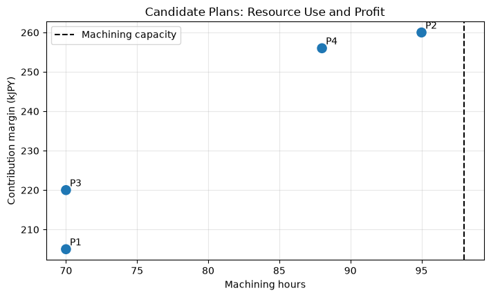
First, create multiple candidate plans and list whether they meet your capabilities and how much profit you can offer.

candidates = pd.DataFrame({"plan": ["current practice", "Avalue", "Bvalue", "Balance proposal"],
                           "A": [25, 40, 20, 32], "B": [20, 15, 30, 24]})
candidates["machining_h"] = 2*candidates["A"] + candidates["B"]
candidates["assembly_h"] = candidates["A"] + 2*candidates["B"]
candidates["profit_kJPY"] = 5*candidates["A"] + 4*candidates["B"]
candidates["feasible"] = ((candidates["machining_h"] <= capacity["machining_h"]) &
                           (candidates["assembly_h"] <= capacity["assembly_h"]))
display(candidates)

colors = candidates["feasible"].map({True: "tab:blue", False: "tab:red"})
plt.scatter(candidates["machining_h"], candidates["profit_kJPY"], c=colors, s=90)
for i, (_, r) in enumerate(candidates.iterrows(), start=1):
    plt.annotate(f"P{i}", (r["machining_h"], r["profit_kJPY"]), xytext=(4,4), textcoords="offset points")
plt.axvline(capacity["machining_h"], color="black", linestyle="--", label="Machining capacity")
plt.title("Candidate Plans: Resource Use and Profit")
plt.xlabel("Machining hours")
plt.ylabel("Contribution margin (kJPY)")
plt.grid(True, alpha=.3)
plt.legend()
plt.tight_layout()
plt.show()

	plan	A	B	machining_h	assembly_h	profit_kJPY	feasible
0	current practice	25	20	70	65	205	True
1	Avalue	40	15	95	70	260	True
2	Bvalue	20	30	70	80	220	True
3	Balance proposal	32	24	88	80	256	True

Reading the results

Red candidates may seem profitable but cannot be hired if they exceed their capabilities. The first step in optimization is to distinguish between the quality of the idea and its feasibility. Since only a few human-created candidates can cause you to miss the best option, the entire candidate space will be examined from now on.

No.002: What is an objective function?

Meaning in Practice

The objective function quantifies “what you want to improve.” If you use marginal profit instead of sales, production decisions will be made after deducting variable costs. However, there are designs that include deadlines and quality objectives, so choosing KPIs is a management decision.

Approach to Analysis and Modeling

If we $p_i$ product-specific marginal profit and production volume $x_i$, the total marginal profit is $f(x)=\sum_i p_ix_i$. The coefficient represents “how much the target value increases when one unit is produced.”

Check with Python

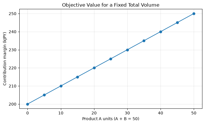
Compare the impact of differences in profit factors on the target value with the same total production volume.

mix = pd.DataFrame({"A": np.arange(0, 51, 5)})
mix["B"] = 50 - mix["A"]
mix["profit_kJPY"] = 5*mix["A"] + 4*mix["B"]
display(mix)
plt.plot(mix["A"], mix["profit_kJPY"], marker="o")
plt.title("Objective Value for a Fixed Total Volume")
plt.xlabel("Product A units (A + B = 50)")
plt.ylabel("Contribution margin (kJPY)")
plt.grid(True, alpha=.3)
plt.tight_layout()
plt.show()

	A	B	profit_kJPY
0	0	50	200
1	5	45	205
2	10	40	210
3	15	35	215
4	20	30	220
5	25	25	225
6	30	20	230
7	35	15	235
8	40	10	240
9	45	5	245
10	50	0	250

Reading the results

Even if the total quantity is the same, the higher the profit coefficient A increases, the higher the target value will be. However, since A requires a lot of processing time, you cannot make everything A based solely on the objective function. You need to look at both purpose and constraints at the same time.

No.003: What Are Constraints

Meaning in Practice

Constraints include equipment capacity, personnel, materials, demand, and safety standards, which the plan must adhere to. If you don’t distinguish between the goal of ‘protect if possible’ and the upper limit of ‘must protect,’ solutions won’t be usable on the ground.

Approach to Analysis and Modeling

The constraints on processing and assembly are as follows.

$2x_A+x_B\le C_M,\qquad x_A+2x_B\le C_A$

The left side shows resource usage, and the right side shows available amounts. Difference $C-Ax$ is the slack and indicates the tightness of the constraint.

Check with Python

plan = pd.Series({"A": 32, "B": 24})
usage = pd.Series({"machining_h": 2*plan["A"] + plan["B"],
                   "assembly_h": plan["A"] + 2*plan["B"]})
constraint_check = pd.DataFrame({"usage": usage, "capacity": capacity})
constraint_check["slack"] = constraint_check["capacity"] - constraint_check["usage"]
constraint_check["utilization_pct"] = 100*constraint_check["usage"]/constraint_check["capacity"]
display(constraint_check)
constraint_check[["usage", "capacity"]].plot(kind="bar")
plt.title("Resource Usage versus Capacity")
plt.xlabel("Resource")
plt.ylabel("Hours")
plt.grid(True, axis="y", alpha=.3)
plt.tight_layout()
plt.show()

	usage	capacity	slack	utilization_pct
machining_h	88	98	10	89.80
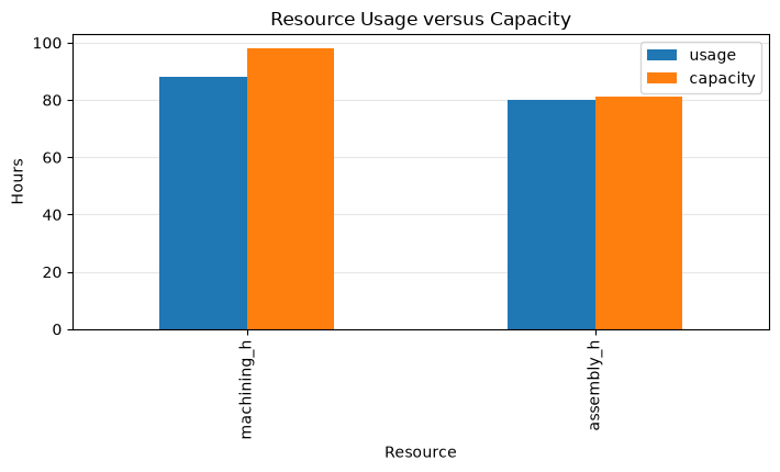
assembly_h	80	81	1	98.77

Reading the results

If your remaining energy is negative, it’s over capacity; if it’s close to zero, you’re a potential bottleneck. Constraints are not only for “increasing utilization rates” but also serve as a basis for discussing which resources to increase to increase planning freedom.

No.004: What is a determinant variable?

Meaning in Practice

Decision variables are values that meetings or systems can actually change. Demand and facility capacity are usually input conditions rather than determinants. Here, $x_A,x_B$ is used as the monthly production volume.

Approach to Analysis and Modeling

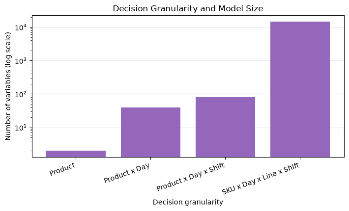
The granularity of variables is important. If you only look at the quantity by product, there are two variables, but if you break it down by day, line, or shift, the numbers surge. Granularity unnecessary for decision-making increases computational load and maintenance burdens.

Check with Python

Compare the scale when variables are subdivided by product into “product× shift.”

scales = pd.DataFrame({
    "model": ["Product", "Product x Day", "Product x Day x Shift", "SKU x Day x Line x Shift"],
    "variables": [2, 2*20, 2*20*2, 120*20*3*2],
})
display(scales)
plt.bar(scales["model"], scales["variables"], color="tab:purple")
plt.yscale("log")
plt.title("Decision Granularity and Model Size")
plt.xlabel("Decision granularity")
plt.ylabel("Number of variables (log scale)")
plt.xticks(rotation=20, ha="right")
plt.grid(True, axis="y", alpha=.3)
plt.tight_layout()
plt.show()

	model	variables
0	Product	2
1	Product x Day	40
2	Product x Day x Shift	80
3	SKU x Day x Line x Shift	14400

Reading the results

Increasing granularity allows for detailed representation of reality, but complicates data organization, calculation, and explanation. Initially, value should be confirmed at the minimum granularity necessary for management decisions, and then variables should be increased when planning or shift constraints become necessary.

No.005: What is a Executable Solution?

Meaning in Practice

An executable solution is a plan that satisfies all constraints simultaneously. Even if profits are high, breaking even one constraint makes it impossible to execute. If there is no viable solution, conditions such as delivery time, capacity, and lower demand may be inconsistent.

Approach to Analysis and Modeling

The set of points that satisfy the constraint is called the executable region. In linear constraints, the region becomes polygonal, and the optimal solution usually appears at its boundaries, especially at vertices.

Check with Python

a_grid = np.arange(0, 51)
b_grid = np.arange(0, 46)
grid = pd.DataFrame([(a,b) for a in a_grid for b in b_grid], columns=["A","B"])
grid["feasible"] = ((2*grid["A"] + grid["B"] <= capacity["machining_h"]) &
                    (grid["A"] + 2*grid["B"] <= capacity["assembly_h"]))
print(f"Grid candidates: {len(grid):,}; feasible: {grid['feasible'].sum():,}")
plt.scatter(grid.loc[grid.feasible,"A"], grid.loc[grid.feasible,"B"], s=8, alpha=.45, label="Feasible")
plt.scatter(grid.loc[~grid.feasible,"A"], grid.loc[~grid.feasible,"B"], s=5, alpha=.08, color="gray", label="Infeasible")
plt.title("Feasible Region of Production Plans")
plt.xlabel("Product A units")
plt.ylabel("Product B units")
plt.grid(True, alpha=.3)
plt.legend()
plt.tight_layout()
plt.show()

Grid candidates: 2,346; feasible: 1,359

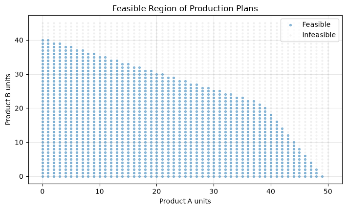
Reading the results

The dark areas are planned to simultaneously meet both process capacity and demand ceilings. Visualizing where the current plan is within this area makes it easier to explain the potential for increased production and the trade-offs to stakeholders.

No.006: What is the optimal solution?

Meaning in Practice

The optimal solution is the one with the best objective function among the executable solutions. “Computational optimization” and “plans to be adopted on site” are not synonymous; adoption is made after checking for factors outside the model and data errors.

Approach to Analysis and Modeling

linprog solves the minimization, so the sign of the profit factor is inverted to minimize $-5x_A-4x_B$. Since it is solved as a continuous variable, be careful that fractions may appear.

Check with Python

c = -products["margin_kJPY"].to_numpy()
A_ub = np.array([[2,1], [1,2]])
b_ub = capacity[["machining_h","assembly_h"]].to_numpy()
bounds = [(0, products.loc["A","demand_limit"]), (0, products.loc["B","demand_limit"])]
res = linprog(c, A_ub=A_ub, b_ub=b_ub, bounds=bounds, method="highs")
optimal = pd.Series(res.x, index=["A","B"], name="optimal_units")
summary = pd.DataFrame({"optimal_units": optimal,
                        "unit_margin_kJPY": products["margin_kJPY"]})
summary["margin_kJPY"] = summary["optimal_units"]*summary["unit_margin_kJPY"]
display(summary)
print(f"Maximum contribution margin: {-res.fun:,.2f} kJPY")

feasible_grid = grid[grid.feasible].copy()
feasible_grid["profit"] = 5*feasible_grid["A"] + 4*feasible_grid["B"]
plt.scatter(feasible_grid["A"], feasible_grid["B"], c=feasible_grid["profit"], s=12, cmap="viridis")
plt.scatter(*res.x, marker="*", s=220, color="red", label="Continuous optimum")
plt.colorbar(label="Contribution margin (kJPY)")
plt.title("Objective Value over the Feasible Region")
plt.xlabel("Product A units")
plt.ylabel("Product B units")
plt.grid(True, alpha=.3)
plt.legend()
plt.tight_layout()
plt.show()

	optimal_units	unit_margin_kJPY	margin_kJPY
A	38.33	5.00	191.67
B	21.33	4.00	85.33

Maximum contribution margin: 277.00 kJPY

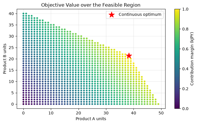
Reading the results

The star mark is the optimal solution for the continuous model. Since it depends on how both resources are used and the balance of product-specific profits, it differs from the plan of “only producing the higher-priced A.” If fractional production is impossible, you need the discrete model No.009.

No.007: Local Optimization and Global Optimization

Meaning in Practice

Local optimization is a better solution than nearby candidates, while global optimization is the best solution among all candidates. For nonlinear issues such as setup count, maintenance cycle, and temperature conditions, exploration may stall at improvements near the initial proposal.

Approach to Analysis and Modeling

Consider a non-convex function with multiple valleys. Local search depends on the starting point, so multiple initials, region division, global search, and lower bound evaluation are required.

Check with Python

t = np.linspace(1, 30, 1000)
cost = 0.035*(t-18)**2 + 2.2*np.sin(t/2.2) + 12
local_idx = np.where((cost[1:-1] < cost[:-2]) & (cost[1:-1] < cost[2:]))[0] + 1
mins = pd.DataFrame({"interval_days": t[local_idx], "cost_index": cost[local_idx]}).sort_values("cost_index")
display(mins.round(2))
plt.plot(t, cost)
plt.scatter(t[local_idx], cost[local_idx], color="tab:red", zorder=3, label="Local minima")
g = local_idx[np.argmin(cost[local_idx])]
plt.scatter(t[g], cost[g], marker="*", s=220, color="gold", edgecolor="black", label="Global minimum")
plt.title("Non-convex Maintenance Interval Cost")
plt.xlabel("Maintenance interval (days)")
plt.ylabel("Cost index")
plt.grid(True, alpha=.3)
plt.legend()
plt.tight_layout()
plt.show()

	interval_days	cost_index
1	23.35	10.96
0	11.42	11.56

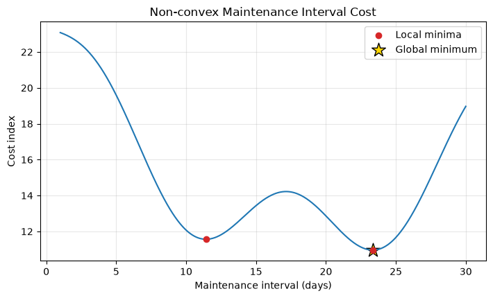
Reading the results

All red dots are locally optimal that cannot be improved in the neighborhood, but only the star is the global optimal for the entire search range. While “gradually changing conditions” improvements on site are effective, starting conditions may cause you to miss other valleys.

No.008: Convex and Non-Convex Optimization

Meaning in Practice

In convex optimization, local optimization becomes global optimization, making it easier to explain the reliability of solutions. Non-convexity arises from fixed costs, scheduling, complex physical properties, integer conditions, and so on.

Approach to Analysis and Modeling

A convex function has a line segment connecting any two points above the function and has a single valley. On the other hand, non-convex functions can have multiple valleys. In modeling, we consider whether convex and linearization can be achieved within a range that does not compromise reality.

Check with Python

x = np.linspace(-4, 6, 600)
convex = (x-1)**2 + 2
nonconvex = 0.08*(x-1)**4 - 1.4*(x-1)**2 + 5
fig, axes = plt.subplots(1, 2, figsize=(10, 4))
axes[0].plot(x, convex, color="tab:blue")
axes[0].set_title("Convex Objective")
axes[1].plot(x, nonconvex, color="tab:orange")
axes[1].set_title("Non-convex Objective")
for ax in axes:
    ax.set_xlabel("Decision variable")
    ax.set_ylabel("Objective value")
    ax.grid(True, alpha=.3)
fig.tight_layout()
plt.show()
print("Convex minimum x =", x[np.argmin(convex)].round(3))
print("Non-convex grid minimum x =", x[np.argmin(nonconvex)].round(3))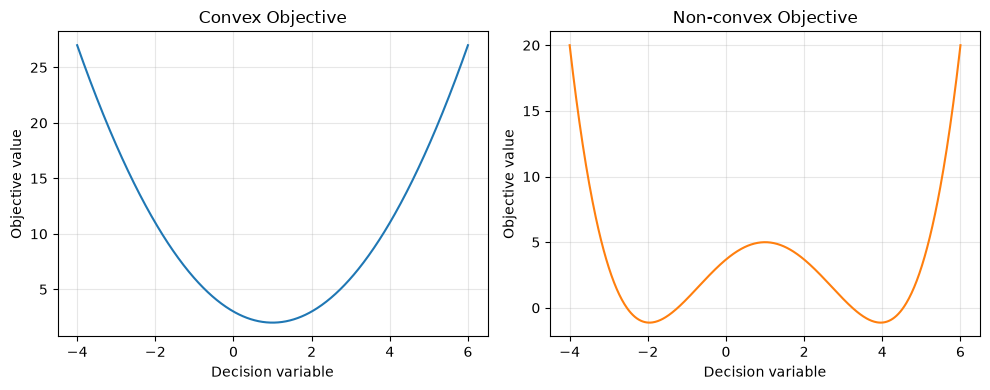

Convex minimum x = 0.992
Non-convex grid minimum x = -1.963

Reading the results

On the left, no matter where you descend, you head into the same valley. The right side has multiple valleys, so you need to pay attention to the solution method and initial values. In practice, not only the “optimal value” but also the optimal guarantee, calculation time, and approximate error are reported.

No.009: Continuous Optimization and Discrete Optimization

Meaning in Practice

If production volume can be handled with any real number at will, continuous optimization is used; if decisions are made by integers or 0/1, such as lot size, equipment acceptance or notification, or the allocation of the person in charge, discrete optimization is used. Simply rounding consecutive solutions leads to constraint violations and loss of profit opportunities.

Approach to Analysis and Modeling

Here, let’s assume you are making a batch of 5 lots of A and 4 lots of B. $x_A=5n_A, x_B=4n_B$ is expressed using the integer lot number $n_A,n_B$.

Check with Python

lot_a, lot_b = 5, 4
lot_plans = pd.DataFrame([(na, nb, lot_a*na, lot_b*nb)
                          for na in range(11) for nb in range(12)],
                         columns=["lots_A","lots_B","A","B"])
lot_plans = lot_plans[(2*lot_plans.A + lot_plans.B <= capacity["machining_h"]) &
                      (lot_plans.A + 2*lot_plans.B <= capacity["assembly_h"])]
lot_plans["profit_kJPY"] = 5*lot_plans.A + 4*lot_plans.B
best_lot = lot_plans.nlargest(5, "profit_kJPY")
display(best_lot)
comparison = pd.DataFrame({
    "plan": ["Continuous optimum", "Best lot plan"],
    "A": [res.x[0], best_lot.iloc[0].A],
    "B": [res.x[1], best_lot.iloc[0].B],
    "profit_kJPY": [-res.fun, best_lot.iloc[0].profit_kJPY],
})
display(comparison)
plt.bar(comparison["plan"], comparison["profit_kJPY"], color=["tab:blue","tab:green"])
plt.title("Continuous versus Lot-based Plan")
plt.xlabel("Model type")
plt.ylabel("Contribution margin (kJPY)")
plt.grid(True, axis="y", alpha=.3)
plt.tight_layout()
plt.show()

	lots_A	lots_B	A	B	profit_kJPY
100	8	4	40	16	264
110	9	2	45	8	257
89	7	5	35	20	255
99	8	3	40	12	248
78	6	6	30	24	246

	plan	A	B	profit_kJPY
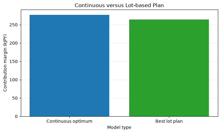
0	Continuous optimum	38.33	21.33	277.00
1	Best lot plan	40.00	16.00	264.00

Reading the results

If you include lot constraints, the candidates may jump too far, and the target value may be lower than that of continuous models. This difference is the price of reality. Continuous solutions are useful as upper limits or benchmarks, but the execution plan recalculates including discrete conditions.

No.010: Situations Where Mathematical Optimization Is Used in Manufacturing

Meaning in Practice

Optimization can be used not only for production quantities but also for selecting order, logistics, inventory, personnel, maintenance, and investment. The key is not to start with the solution, but to clarify the frequency of decisions, who is responsible, input data, and post-output operations.

Approach to Analysis and Modeling

Candidates for application can be evaluated based on “economic effect,” “data readiness,” “decision frequency,” and “clarity of constraints.” Even if the effect is significant, if the data and operations are not yet well established, it is not suitable for short-term implementation.

Check with Python

use_cases = pd.DataFrame({
    "use_case": ["Production mix", "Scheduling", "Inventory", "Workforce", "Maintenance", "Capital investment"],
    "business_value": [9, 9, 8, 7, 7, 9],
    "data_readiness": [8, 6, 8, 7, 6, 5],
    "decision_frequency": [8, 9, 8, 9, 7, 3],
})
use_cases["priority_score"] = (0.45*use_cases.business_value +
                               0.35*use_cases.data_readiness +
                               0.20*use_cases.decision_frequency)
display(use_cases.sort_values("priority_score", ascending=False))
plt.scatter(use_cases.data_readiness, use_cases.business_value,
            s=60*use_cases.decision_frequency, alpha=.7)
for _, r in use_cases.iterrows():
    plt.annotate(r.use_case, (r.data_readiness, r.business_value), xytext=(4,4), textcoords="offset points")
plt.title("Optimization Use-case Portfolio")
plt.xlabel("Data readiness score")
plt.ylabel("Business value score")
plt.xlim(0, 10); plt.ylim(0, 10)
plt.grid(True, alpha=.3)
plt.tight_layout()
plt.show()

	use_case	business_value	data_readiness	decision_frequency	priority_score
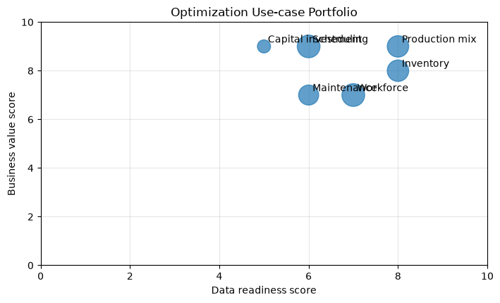
0	Production mix	9	8	8	8.45
2	Inventory	8	8	8	8.00
1	Scheduling	9	6	9	7.95
3	Workforce	7	7	9	7.40
4	Maintenance	7	6	7	6.65
5	Capital investment	9	5	3	6.40

Reading the results

In this hypothetical evaluation, production allocation and inventory are candidates that are easier to start in terms of both effectiveness and readiness. The size of the dots reflects the frequency of judgments, and repeated daily and weekly judgments indicate that the effects of systematization tend to accumulate more easily. In actual projects, stakeholders agree on evaluation criteria and weighting.

Practical Implications Seen Through Target Exercise

The value of mathematical optimization lies not only in the optimal solution itself. During the process of determining objective functions, you can align the evaluation axes between departments and visualize implicit operational rules by listing constraints. Additionally, by checking the gap between capacity and target values, we can quantify discussions about capacity enhancement, outsourcing, and demand adjustment.

On the other hand, the model is a representation of reality. If quality risks, equipment failures, skill gaps, urgent orders, and other information are not entered into the solution, they will not be reflected in the solution. It is important not to overtrust the word “optimal,” but to design proposals that are adoptable and to provide decision-making support that presents their rationale, assumptions, and sensitivity.

What is necessary for practical implementation

1. Definition of decision-making: Decide who, when, and what to decid, and which KPIs to evaluate
2. Data definition: Align capacity, standard time, profit, demand, inventory granularity, update frequency, and responsible departments
3. Inventory of constraints: Separate records of physical constraints, contract terms, quality and safety, and on-site practices
4. Comparison with the Current Plan: Compare not only objective values but also feasibility, stability, and explainability
5. Sensitivity Analysis and Exception Operations: Decide on procedures for changes in demand or capacity and emergency personnel for correction
6. Small Demonstration: Limit target products and durations to verify improvements in planning time and performance KPIs

Conclusion

From No.001 to No.010, the objective functions, constraints, determinants, executable solutions, and optimal solutions that make up mathematical optimization were checked using the production allocation of a hypothetical factory. Furthermore, by classifying them into local/global, convex/non-convex, and continuous/discrete, we observed that the solution method and optimal guarantee vary depending on the nature of the problem.

The starting point in practice is not advanced solutions, but whether decisions can be translated into these three elements. In the next phase, small-scale verification—including comparisons with current operations, data quality, and exception handling—increases the chances of success.

Consultations for Corporations

At Suri Kobo, we support data analysis and mathematical optimization design, PoC, and business implementation for manufacturing decision-making, including production planning, scheduling, inventory and logistics, staffing allocation, and capital investment. Even if the issue is not yet formulated, you can consult with us starting from business interviews and data inventory.

📩 Contact Us: surikobo.co.jp/contact
Please feel free to consult us first.