Reducing Delivery Delays in Realistic Time: 10 Exercises to Optimize Production Sequences

Using a hypothetical multi-variety, small-lot production line as the subject, we compare the use of exact and approximate solutions, greedy methods, local searches, annealing methods, genetic algorithms, taboo searches, particle swarm optimization, and large-scale neighborhood searches. The target is No.081〜No.090(Heuristics, Metaheuristics).

[!NOTE] This material is a notebook previously used by Surikoubo (or personally by the representative, Kazuyama), and has been reconstructed, edited, and published with the company’s permission. All data listed is fictional and has no relation whatsoever to real companies, factories, or figures.

Introduction: Practical Challenges in Manufacturing Covered in This Article

On lines where processing time, delivery time, and importance differ from order to order, simply changing the order of input can significantly affect delivery delays. This paper deals with problems that determine the order for suppressing total weighted delay within a limited calculation time.

Common situations on site

• After the morning assembly, express items, equipment stoppages, and vacancies arise, so plans are reorganized
• You want to give instructions to the site within minutes, but the candidate order increases by multiplying the number of jobs.
• Delivery time, stability, and explainability are prioritized over the word “optimal.”

Why is this issue so difficult to judge?

$n$ order is $n!$ as follows. With 8 cases, that’s 40,320 ways, but with 20 items, that’s about $2.43\times10^{18}$ ways. Also, even if the target values are the same, the planning and impact on key customers differ, so operational design that includes computation time and solution quality is necessary.

Overview of Exercise covered this time

No.	Theme	Questions on the Ground
081	Exact Solutions and Approximate Solutions	How much optimization is guaranteed?
082	heuristics	How to turn business knowledge into an initial plan
083	Greed law	Can you quickly establish the order by making sequential judgments?
084	Local Exploration Method	Can Replacing Nearby Areas Improve Issues
085	annealing method	Can we allow temporary deterioration and get over the valley?
086	Genetic algorithm	Can you make use of combinations with multiple candidates?
087	taboo search	Can we prevent loops to the same solution?
088	Particle Swarm Optimization	Can you search for a good order from continuous expression?
089	Large-scale Neighborhood Search	Can you break part of the order and redo it?
090	Commitment to Precision	How to choose solutions sufficient for decision-making

Preparing the Python environment

No external data is used; random number seeds are fixed. For fairness in comparison, the same evaluation function is used across all methods. Graphs are created using Matplotlib.

import platform, time, itertools, math
import numpy as np
import pandas as pd
import matplotlib
import matplotlib.pyplot as plt
from IPython.display import display

SEED = 42
rng = np.random.default_rng(SEED)
plt.rcParams["figure.figsize"] = (7.4, 4.5)
plt.rcParams["font.size"] = 10
print("Python:", platform.python_version())
print("numpy:", np.__version__, "pandas:", pd.__version__, "matplotlib:", matplotlib.__version__)

Python: 3.13.1
numpy: 2.5.1 pandas: 3.0.3 matplotlib: 3.11.0

Creation of Fictional Data

A single bottleneck machine can continuously process 8 jobs. Job $j$ machining time $p_j$, deadline $d_j$, importance $w_j$, completion time $C_j$, and KPI weighted delay

$F(\pi)=\sum_{j=1}^{n} w_j\max(C_j-d_j,0)$

Let’s say so. The smaller, the better, and the unit is “weighted importance time.” For a concise comparison, this article omits the setup time.

jobs = pd.DataFrame({
    "job": list("ABCDEFGH"),
    "processing_h": [5, 8, 4, 7, 3, 9, 6, 5],
    "due_h": [14, 18, 11, 27, 9, 35, 23, 20],
    "priority": [3, 5, 2, 4, 6, 2, 5, 3],
})
p = jobs.processing_h.to_numpy(); due = jobs.due_h.to_numpy(); weight = jobs.priority.to_numpy(); n = len(jobs)

def score(order):
    order = np.asarray(order, dtype=int)
    completion = np.cumsum(p[order])
    return int(np.sum(weight[order] * np.maximum(completion - due[order], 0)))

def schedule(order):
    order = np.asarray(order, dtype=int); completion = np.cumsum(p[order])
    return pd.DataFrame({"sequence": np.arange(1, n+1), "job": jobs.job.to_numpy()[order],
                         "completion_h": completion, "due_h": due[order],
                         "tardiness_h": np.maximum(completion-due[order], 0), "priority": weight[order]})

display(jobs)
print("Number of candidate ordinals:", math.factorial(n))

	job	processing_h	due_h	priority
0	A	5	14	3
1	B	8	18	5
2	C	4	11	2
3	D	7	27	4
4	E	3	9	6
5	F	9	35	2
6	G	6	23	5
7	H	5	20	3

Number of candidates: 40320

No.081: Exact Solutions and Approximate Solutions

Meaning in Practice

Exact solutions guarantee optimization, but as the number of cases increases, calculations may not be completed. Instead of loosening guarantees, the approximate solution returns a good plan within a practical timeframe.

Approach to Analysis and Modeling

This time, we will seek a strict $F^*$ by listing all the methods and measure the quality of subsequent methods using gap $(F-F^*)/F^*\times100$. All listings are for small-scale verification and are not standard solutions for large-scale problems.

Check with Python

t0 = time.perf_counter(); exact_order = min(itertools.permutations(range(n)), key=score); exact_sec = time.perf_counter()-t0
exact_score = score(exact_order)
display(schedule(exact_order))
print("exact solution:", "-".join(jobs.job.iloc[list(exact_order)]), "Target value:", exact_score, "calculation second:", round(exact_sec, 4))

	sequence	job	completion_h	due_h	tardiness_h	priority
0	1	C	4	11	0	2
1	2	E	7	9	0	6
2	3	A	12	14	0	3
3	4	B	20	18	2	5
4	5	G	26	23	3	5
5	6	H	31	20	11	3
6	7	D	38	27	11	4
7	8	F	47	35	12	2

Exact solution: C-E-A-B-G-H-D-F Objective value: 126 Calculation second: 0.1657

Reading the results

All 8 items can be listed to obtain the optimal value for comparison. On the other hand, as the number of cases increases, the number of listings surges. It is realistic to calibrate the approximation method on small instances and set a time limit at production scale.

No.082: What is heuristics?

Meaning in Practice

Heuristics turns on-site empirical rules into reproducible calculation procedures. Metrics that consider Fastest Delivery (EDD) and priority are easy-to-explain initial proposals.

Approach to Analysis and Modeling

A single rule is not necessarily optimal for every KPI. EDD, short-time order (SPT), and $d_j/w_j$ order are evaluated using the same objective function.

Check with Python

t0=time.perf_counter()
rules={"EDD":np.argsort(due), "SPT":np.argsort(p), "due/priority":np.argsort(due/weight)}
rows=[]
for name,o in rules.items(): rows.append([name,"-".join(jobs.job.iloc[o]),score(o)])
heuristic_sec=time.perf_counter()-t0
heuristic_df=pd.DataFrame(rows,columns=["rule","order","objective"]).sort_values("objective")
display(heuristic_df)

	rule	order	objective
0	EDD	E-C-A-B-H-G-D-F	133
1	SPT	E-C-A-H-G-D-B-F	136
2	due/priority	E-B-G-A-C-H-D-F	155

Reading the results

The results vary depending on the rules. It is important to select rules that align with the objective KPIs and to record exception handling without leaving it as tacit knowledge.

No.083: The Method of Greed

Meaning in Practice

The Greedy Method selects the best next job at each point and completes the entire sequence in a short time. This is the initial solution for emergency replanning.

Approach to Analysis and Modeling

Select candidates with the smallest incremental delay when adding one pending job to the end. If there is a tie, priority will be given to the faster delivery date. However, the future impact is not fully foreseeable.

Check with Python

def greedy():
    order=[]; remaining=set(range(n))
    while remaining:
        j=min(remaining,key=lambda x:(score(order+[x]),due[x],p[x]))
        order.append(j); remaining.remove(j)
    return np.array(order)
t0=time.perf_counter(); greedy_order=greedy(); greedy_sec=time.perf_counter()-t0
display(schedule(greedy_order))
print("Greed and desire are satisfied.:", score(greedy_order))

	sequence	job	completion_h	due_h	tardiness_h	priority
0	1	E	3	9	0	6
1	2	C	7	11	0	2
2	3	A	12	14	0	3
3	4	H	17	20	0	3
4	5	G	23	23	0	5
5	6	F	32	35	0	2
6	7	D	39	27	12	4
7	8	B	47	18	29	5

Greed Relief: 193

Reading the results

You can instantly return actionable proposals, but you can’t revoke your early decisions later. Using this solution as a starting point for local exploration makes it easier to balance speed and quality.

No.084: Local Exploration Method

Meaning in Practice

By repeatedly making small changes to existing plans, you can gradually improve plan changes.

Approach to Analysis and Modeling

2. Search all nearby areas where you want to swap positions, and move if the best improvement is available. If there is no improvement within the neighborhood, local optimization is considered good, but it is not necessarily global optimal.

Check with Python

def local_search(start):
    cur=np.array(start).copy(); history=[score(cur)]
    while True:
        best=cur; best_s=score(cur)
        for i in range(n-1):
            for j in range(i+1,n):
                cand=cur.copy(); cand[i],cand[j]=cand[j],cand[i]
                if score(cand)<best_s: best,best_s=cand,score(cand)
        if best_s>=score(cur): break
        cur=best.copy(); history.append(best_s)
    return cur,history
t0=time.perf_counter(); local_order,local_hist=local_search(greedy_order); local_sec=time.perf_counter()-t0
plt.plot(local_hist,marker="o"); plt.title("Local search convergence"); plt.xlabel("Iteration"); plt.ylabel("Weighted tardiness"); plt.grid(True); plt.tight_layout(); plt.show()
print("Local Exploration Solution:",score(local_order),"Repeatedly:",len(local_hist)-1)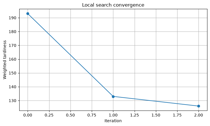

Local exploration solutions: 126 Repetitions: 2

Reading the results

Desired values improve from greed solutions, and the improvement process can be tracked. By changing multiple initial solutions or adding insertion neighborhoods, you can reduce dependence on local optimization.

No.085: Annealing Method

Meaning in Practice

The annealing method allows for temporary deterioration in the early stages to escape local optimalization, and focuses on improvement in the final stages.

Approach to Analysis and Modeling

Accept candidates with a deterioration $\Delta>0$ with a probability of $\exp(-\Delta/T)$ and gradually lower the temperature $T$. You can reproduce by saving random seed numbers, initial temperature, and cooling rate.

Check with Python

def anneal(start,seed=SEED,steps=2500):
    r=np.random.default_rng(seed); cur=np.array(start).copy(); best=cur.copy(); hist=[]
    for k in range(steps):
        T=40*(0.002**(k/(steps-1))); i,j=r.choice(n,2,replace=False); cand=cur.copy(); cand[i],cand[j]=cand[j],cand[i]
        delta=score(cand)-score(cur)
        if delta<=0 or r.random()<np.exp(-delta/T): cur=cand
        if score(cur)<score(best): best=cur.copy()
        hist.append(score(best))
    return best,hist
t0=time.perf_counter(); sa_order,sa_hist=anneal(greedy_order); sa_sec=time.perf_counter()-t0
plt.plot(sa_hist); plt.title("Simulated annealing: best-so-far"); plt.xlabel("Iteration"); plt.ylabel("Weighted tardiness"); plt.grid(True); plt.tight_layout(); plt.show()
print("annealing solution:",score(sa_order))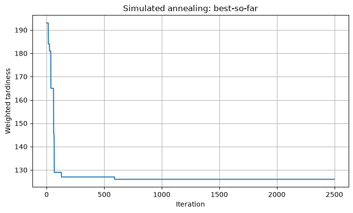

Annealing Solution: 126

Reading the results

If you save the best-so-far, you won’t lose the best option even if you accept a deterioration solution midway. Confirm quality distribution across multiple seeds and evaluate stability within the time limit.

No.086: Genetic Algorithm

Meaning in Practice

We maintain multiple production orders simultaneously and combine good partial orders to explore. A key feature is that it allows for a diverse range of candidates.

Approach to Analysis and Modeling

Create non-duplicate pieces with an ordered cross (OX) and add swap mutations. Elite preservation is the best way to prevent deterioration.

Check with Python

def genetic(seed=SEED,pop_size=40,generations=100):
    r=np.random.default_rng(seed); pop=[r.permutation(n) for _ in range(pop_size)]; hist=[]
    for _ in range(generations):
        pop=sorted(pop,key=score); new=[pop[0].copy(),pop[1].copy()]
        while len(new)<pop_size:
            a,b=r.choice(pop[:15],2,replace=False); lo,hi=sorted(r.choice(n,2,replace=False)); child=np.full(n,-1); child[lo:hi]=a[lo:hi]
            fill=[x for x in b if x not in child]; child[child<0]=fill
            if r.random()<.25: i,j=r.choice(n,2,replace=False); child[i],child[j]=child[j],child[i]
            new.append(child)
        pop=new; hist.append(score(min(pop,key=score)))
    best=min(pop,key=score); return best,hist
t0=time.perf_counter(); ga_order,ga_hist=genetic(); ga_sec=time.perf_counter()-t0
plt.plot(ga_hist); plt.title("Genetic algorithm: best-so-far"); plt.xlabel("Generation"); plt.ylabel("Weighted tardiness"); plt.grid(True); plt.tight_layout(); plt.show()
print("Genetic Algorithm Solutions:",score(ga_order))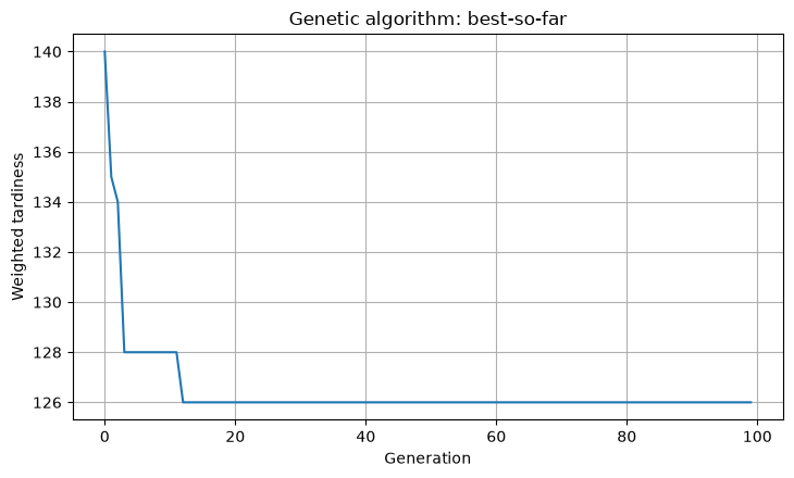

Genetic algorithm solutions: 126

Reading the results

You can see how the best values for each generation converge. If the population is always in the same order, review the mutation rate and how the initial population is created.

No.087: Taboo Search

Meaning in Practice

Temporary bans on the most recent exchanges will prevent cycles of repeating the same order back and forth. This method makes it easier to maintain broader searches than local searches.

Approach to Analysis and Modeling

Exchange job pairs will be placed on the taboo list for a certain period. However, moving to break the previous best is permitted according to the Aspiration Standard.

Check with Python

def tabu_search(start,iterations=120,tenure=7):
    cur=np.array(start).copy(); best=cur.copy(); tabu={}; hist=[]
    for k in range(iterations):
        candidates=[]
        for i in range(n-1):
            for j in range(i+1,n):
                cand=cur.copy(); moved=tuple(sorted((int(cur[i]),int(cur[j])))); cand[i],cand[j]=cand[j],cand[i]; s=score(cand)
                if tabu.get(moved,-1)<=k or s<score(best): candidates.append((s,cand,moved))
        s,cur,moved=min(candidates,key=lambda x:x[0]); tabu[moved]=k+tenure
        if s<score(best): best=cur.copy()
        hist.append(score(best))
    return best,hist
t0=time.perf_counter(); tabu_order,tabu_hist=tabu_search(greedy_order); tabu_sec=time.perf_counter()-t0
plt.plot(tabu_hist); plt.title("Tabu search: best-so-far"); plt.xlabel("Iteration"); plt.ylabel("Weighted tardiness"); plt.grid(True); plt.tight_layout(); plt.show()
print("Taboo Search Solution:",score(tabu_order))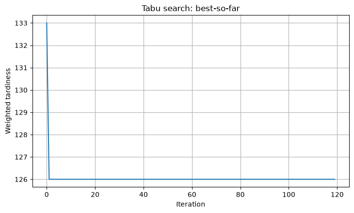

Taboo Search Solutions: 126

Reading the results

You can continue exploring while using movement that doesn’t improve your progress. If the taboo period is too short, it cycles; if too long, exploration flexibility decreases, so verification is conducted according to the scale of the problem.

No.088: Particle Swarm Optimization

Meaning in Practice

Particle Swarm Optimization (PSO) involves each candidate sharing and exploring positive experiences of themselves and the group. It excels at optimizing continuous conditions, and for order problems, creative expression is required.

Approach to Analysis and Modeling

Each job is assigned a priority key for consecutive values, and the order of production is based on the order of production, using the random-key representation. The update speed is $v\leftarrow \omega v+c_1r_1(p-x)+c_2r_2(g-x)$.

Check with Python

def pso(seed=SEED,particles=35,steps=100):
    r=np.random.default_rng(seed); x=r.normal(size=(particles,n)); v=np.zeros_like(x); pb=x.copy(); ps=np.array([score(np.argsort(z)) for z in x]); g=pb[np.argmin(ps)].copy(); hist=[]
    for _ in range(steps):
        v=.72*v+1.4*r.random(x.shape)*(pb-x)+1.4*r.random(x.shape)*(g-x); x+=v
        s=np.array([score(np.argsort(z)) for z in x]); improve=s<ps; pb[improve]=x[improve]; ps[improve]=s[improve]; g=pb[np.argmin(ps)].copy(); hist.append(ps.min())
    return np.argsort(g),hist
t0=time.perf_counter(); pso_order,pso_hist=pso(); pso_sec=time.perf_counter()-t0
plt.plot(pso_hist); plt.title("Particle swarm optimization: best-so-far"); plt.xlabel("Iteration"); plt.ylabel("Weighted tardiness"); plt.grid(True); plt.tight_layout(); plt.show()
print("Particle Swarm Optimization Solutions:",score(pso_order))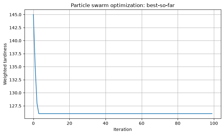

Particle group optimization solution: 126

Reading the results

You can also search the order in PSO as well, but there are flat areas where the order does not change even if the key changes. Do not adopt it without comparing with order-only methods, and check the impact of representation transformation.

No.089: Large-Scale Nearby Search

Meaning in Practice

This is suitable for situations where you need to run multiple jobs together to significantly disrupt part of your plan and redo it. It can also be extended to operations that fix confirmed processes.

Approach to Analysis and Modeling

Three jobs are randomly removed, and while checking all insertion positions, you return them one by one. If the current solution is better, it is used and destroyed and repaired repeatedly.

Check with Python

def lns(start,seed=SEED,iterations=180,destroy=3):
    r=np.random.default_rng(seed); cur=list(start); best=cur.copy(); hist=[]
    for _ in range(iterations):
        removed=list(r.choice(cur,destroy,replace=False)); partial=[x for x in cur if x not in removed]
        for job in removed:
            choices=[partial[:k]+[job]+partial[k:] for k in range(len(partial)+1)]; partial=min(choices,key=score)
        if score(partial)<score(cur): cur=partial
        if score(cur)<score(best): best=cur.copy()
        hist.append(score(best))
    return np.array(best),hist
t0=time.perf_counter(); lns_order,lns_hist=lns(greedy_order); lns_sec=time.perf_counter()-t0
plt.plot(lns_hist); plt.title("Large neighborhood search: best-so-far"); plt.xlabel("Iteration"); plt.ylabel("Weighted tardiness"); plt.grid(True); plt.tight_layout(); plt.show()
print("Large-scale Neighborhood Search Solutions:",score(lns_order))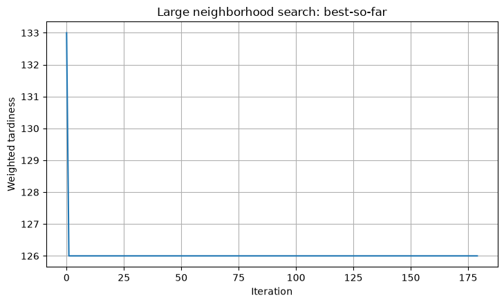

Large-scale Neighborhood Search Solution: 126

Reading the results

You can explore structures that are difficult to overcome with small exchanges through destruction and restoration. In practice, the scope of destruction is adjusted to match operational constraints, such as “not destroying jobs that have already started” or “grouping the same product type.”

No.090: Don’t be overly fixated on strict solutions in practice

Meaning in Practice

Site value is not determined solely by optimality. The method is chosen based on factors such as speed of replanning, solution stability, explainability, and suitability to operational constraints.

Approach to Analysis and Modeling

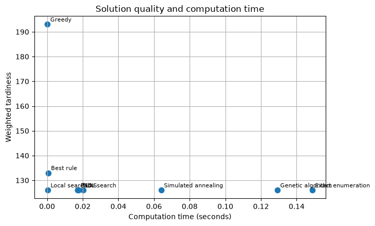
Compare the objective value, difference from the exact solution, and calculation time in the same table. We predefine the allowable gap $\epsilon$ and time limit, and design the end conditions if the best value updates stop.

Check with Python

methods={
 "Exact enumeration":(exact_order,exact_sec), "Best rule":(rules[heuristic_df.iloc[0]["rule"]],heuristic_sec),
 "Greedy":(greedy_order,greedy_sec), "Local search":(local_order,local_sec), "Simulated annealing":(sa_order,sa_sec),
 "Genetic algorithm":(ga_order,ga_sec), "Tabu search":(tabu_order,tabu_sec), "PSO":(pso_order,pso_sec), "LNS":(lns_order,lns_sec)}
comparison=pd.DataFrame([[name,score(o),100*(score(o)-exact_score)/exact_score,sec,"-".join(jobs.job.iloc[list(o)])] for name,(o,sec) in methods.items()],columns=["method","objective","gap_pct","seconds","order"]).sort_values(["objective","seconds"])
display(comparison.round({"gap_pct":2,"seconds":4}))
plt.scatter(comparison.seconds,comparison.objective,s=55)
for _,r in comparison.iterrows(): plt.annotate(r["method"],(r.seconds,r.objective),xytext=(4,4),textcoords="offset points",fontsize=8)
plt.title("Solution quality and computation time"); plt.xlabel("Computation time (seconds)"); plt.ylabel("Weighted tardiness"); plt.grid(True); plt.tight_layout(); plt.show()

	method	objective	gap_pct	seconds	order
3	Local search	126	0.00	0.0004	E-C-A-B-G-H-D-F
6	Tabu search	126	0.00	0.0179	E-C-A-B-G-H-D-F
7	PSO	126	0.00	0.0179	C-E-A-B-G-H-D-F
8	LNS	126	0.00	0.0212	E-C-A-B-G-H-D-F
4	Simulated annealing	126	0.00	0.0682	E-C-A-B-G-H-D-F
5	Genetic algorithm	126	0.00	0.1153	C-E-A-B-G-H-D-F
0	Exact enumeration	126	0.00	0.1657	C-E-A-B-G-H-D-F
1	Best rule	133	5.56	0.0005	E-C-A-B-H-G-D-F
2	Greedy	193	53.17	0.0002	E-C-A-H-G-F-D-B

Reading the results

In this small-scale example, you can identify gaps in each method using the exact solution as the standard. In actual production, acceptance criteria are set on a business basis, for example, “within 60 seconds, improvement of 10% or more from the standard plan, fixed fixed tasks.” If instructions are delayed or plans frequently change due to small target price differences, operational value should be prioritized over rigor.

Practical Implications Seen Through Target Exercise

• Exact solutions are effective as a benchmark for verifying approximation methods with small-scale data.
• Greedy methods provide fast initial solutions, local search provides lightweight improvements, and metaheuristics can be used for locally optimal escapes.
• The random method not only fixes the seed but also evaluates the distribution of target values and required time across multiple seeds.
• Include not only objective values but also calculation time, plan change volume, constraint violations, and explainability as operational KPIs.
• Save and reproducible the best solution, search history, parameters, and input data versions.

What is necessary for practical implementation

Points of Contention	confirmation item	deliverable
objective function	Lost by one hour of delay, customer priority, and setup costs	KPI Definition Book
restriction	Equipment, personnel, planning, breaks, fixed tasks	List of Restrictions and Exceptions
Quality Standards	Allowable gaps, reference plan ratios, calculation time limits	acceptance criteria
Stable operation	Multiple seeds, rule resolution during failures, manual fixes	Operation Procedure Manual
Collaboration	Order and actual data, plan confirmation time, output destination	Data Specifications and API Specifications
surveillance	Actual delays, number of replans, manual revision rates	Monitoring screen

The PoC involves replication tests from past days and blind comparisons by the staff. We check not only the improvement rate but also whether you can return a safe plan in case of input errors or sudden changes.

Conclusion

Heuristics and meta-heuristics are not methods to abandon guarantees of optimality, but rather options to maximize decision value within limited time. It is important to measure quality with small-scale strict solutions and select search methods and termination conditions according to site time constraints and tolerance for change.

Consultations for Corporations

At Suri Kobo, we support optimization of production sequences, equipment and personnel allocation, delivery, and inventory, including problem organization, data diagnosis, PoC, and integration into existing systems. We compare rigorous and approximate methods to design decision-making processes that can be continuously used in the field.

📩 Contact Us: surikobo.co.jp/contact Please feel free to consult us first.