Production planning that resists demand fluctuations: 10-step probability optimization that balances profit, stockouts, and resilience

Using a fictional precision parts factory as the subject, we examine how to determine production volume before demand or yield is finalized. The target is No.071〜No.080(Probability Optimization / Robust Optimization). Not only expected profits, but also out-of-stock probability, worst-case scenarios, CVaR, and balancing profit and CO2 are compared from the same data to differences in decision-making.

[!NOTE] This material is a notebook previously used by Surikoubo (or personally by the representative, Kazuyama), and has been reconstructed, edited, and published with the company’s permission.
All data listed is fictional and has no relation whatsoever to real companies, factories, or figures.

Introduction: Practical Challenges in Manufacturing Covered in This Article

Monthly production volumes may be decided before all orders are finalized. Making more can avoid stockouts, but it increases excess inventory, overtime, and waste. Producing less may seem more efficient, but opportunities can be lost when demand is upset. The purpose of this article is not to “guess a single prediction value,” but to create a plan that can be explained including prediction errors.

Common situations on site

• Sales forecasts change monthly and are finalized later than manufacturing lead times.
• Yield, equipment shutdowns, and the unit price of express materials also fluctuate
• Not only profit maximization, but also targets for on-time delivery rates, overtime, and CO2 emissions
• Plans made solely on average demand run out of stock during busy months and stagnate in slow months

Why is this issue so difficult to judge?

This is because your attitude toward uncertainty can change the “best” plan. You need to agree in advance whether to prioritize average profits, meet demand with a certain probability, or protect the worst-case scenario within the observation range. Additionally, overly conservative planning drives up peacetime costs. Therefore, we judge not only the optimal value but also profit distribution, out-of-stock rate, and sensitivity to assumptions side by side.

Overview of Exercise covered this time

No.	Theme	Questions Answered On-Site
071	Optimization with Uncertainty	What do average-only plans miss?
072	Probability programming	How to Consolidate Profit and Loss by Scenario
073	scenario optimization	How to evaluate the combination of demand and yield
074	Chance constraint	How to Keep the Probability of Out-of-Stock Within an Acceptable Range
075	Robust optimization	How to Meet Worst-Demand Within the Expected Range
076	Distribution-Robust Optimization	How to Prepare for Distribution Estimate Biases
077	Multi-Purpose Optimization	How to handle profits and CO2 simultaneously
078	Pareto is best	How to present alternatives that management can choose from.
079	Risk Scales and CVaR	How to measure losses in bad cases
080	Production planning considering demand fluctuations	How to compare policies and decide on recommended plans

Preparing the Python environment

No external data is used. Fix the random number seed so you can reproduce the same result. The amount is ten thousand yen, the quantity is lot, and the CO2 is kg-CO2. All graphs are created using Matplotlib.

import platform
import numpy as np
import pandas as pd
import matplotlib
import matplotlib.pyplot as plt
from scipy.optimize import minimize_scalar
from scipy.stats import norm
from IPython.display import display

rng = np.random.default_rng(20260712)
plt.rcParams["figure.figsize"] = (8, 4.5)
plt.rcParams["axes.unicode_minus"] = False

print("Python     :", platform.python_version())
print("NumPy      :", np.__version__)
print("pandas     :", pd.__version__)
print("Matplotlib :", matplotlib.__version__)

Python     : 3.13.1
NumPy      : 2.5.1
pandas     : 3.0.3
Matplotlib : 3.11.0

Creation of Fictional Data

We assume a monthly plan for precision parts A. If we $q$ production volume, $D$ demand, and $Y$ yield, the number of good products is $qY$. The selling price is 18,000 yen, normal production costs are 9,000 yen, the disposal value of surplus items is 3,500 yen, and the opportunity loss for out-of-stock is 8,000 yen.

Profit in scenario $s$

$$\pi_s(q)=p\min(qY_s,D_s)+v(qY_s-D_s)_+-c q-b(D_s-qY_s)_+$$

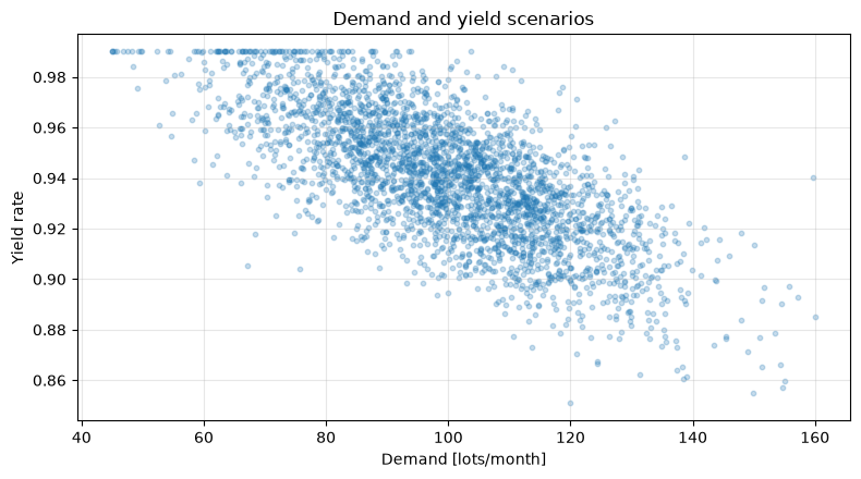
That’s how it is defined. Here is $(x)_+=\max(x,0)$. It creates a weak negative correlation between demand and yield, representing a hypothetical scenario where yield slightly declines during busy periods.

n_scenarios = 3000
z_d = rng.normal(size=n_scenarios)
z_y = rng.normal(size=n_scenarios)
demand = np.clip(100 + 18*z_d, 45, 160)
yield_rate = np.clip(0.94 - 0.018*z_d + 0.018*z_y, 0.84, 0.99)
scenarios = pd.DataFrame({"demand": demand, "yield_rate": yield_rate})

price, unit_cost, salvage, shortage_penalty = 1.80, 0.90, 0.35, 0.80

def profit(q, d=demand, y=yield_rate):
    good = q * y
    sold = np.minimum(good, d)
    surplus = np.maximum(good-d, 0)
    shortage = np.maximum(d-good, 0)
    return price*sold + salvage*surplus - unit_cost*q - shortage_penalty*shortage

display(scenarios.describe(percentiles=[.05, .5, .95]).round(2))

fig, ax = plt.subplots()
ax.scatter(demand, yield_rate, s=10, alpha=.25)
ax.set_title("Demand and yield scenarios")
ax.set_xlabel("Demand [lots/month]")
ax.set_ylabel("Yield rate")
ax.grid(True, alpha=.3)
plt.tight_layout()
plt.show()

	demand	yield_rate
count	3000.00	3000.00
mean	99.77	0.94
std	18.01	0.03
min	45.00	0.85
5%	69.90	0.90
50%	99.73	0.94
95%	129.11	0.98
max	160.00	0.99

No.071: Optimization with Uncertainty

Meaning in Practice

If you plan only on average demand, you ignore the narrowing of demand distribution and yield decline. In optimization involving uncertainty, unknown quantities are treated as random variables or intervals before decision-making, and the performance of the plan is evaluated by distribution.

Approach to Analysis and Modeling

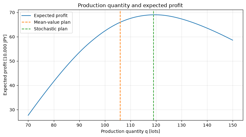
First, compare a fixed plan that substitutes only the average value with a plan that maximizes expected returns across multiple scenarios. Expected value planning is

$\max_q\;\mathbb{E}[\pi(q,D,Y)]$

That’s right. However, even if the expected profit is high, it does not mean the downside risk is small.

Check with Python

q_grid = np.arange(70, 151)
deterministic_profit = [profit(q, np.array([demand.mean()]), np.array([yield_rate.mean()]))[0] for q in q_grid]
expected_profit = np.array([profit(q).mean() for q in q_grid])
q_det = q_grid[np.argmax(deterministic_profit)]
q_sto = q_grid[np.argmax(expected_profit)]

comparison_071 = pd.DataFrame({
    "plan": ["mean-value", "stochastic"],
    "production_q": [q_det, q_sto],
    "expected_profit": [profit(q_det).mean(), profit(q_sto).mean()],
    "shortage_probability": [(q_det*yield_rate < demand).mean(), (q_sto*yield_rate < demand).mean()]
})
display(comparison_071.round(3))

fig, ax = plt.subplots()
ax.plot(q_grid, expected_profit, label="Expected profit")
ax.axvline(q_det, color="tab:orange", linestyle="--", label="Mean-value plan")
ax.axvline(q_sto, color="tab:green", linestyle="--", label="Stochastic plan")
ax.set_title("Production quantity and expected profit")
ax.set_xlabel("Production quantity q [lots]")
ax.set_ylabel("Expected profit [10,000 JPY]")
ax.grid(True, alpha=.3)
ax.legend()
plt.tight_layout()
plt.show()

	plan	production_q	expected_profit	shortage_probability
0	mean-value	106	65.951	0.501
1	stochastic	119	69.028	0.283

Reading the results

Average and probability planning differ in recommended quantities and out-of-stock probabilities. The difference is not a “difference in forecasting accuracy,” but rather the effect of evaluating asymmetric surplus and out-of-stock costs across the entire distribution. On site, the average profit and out-of-stock rate are always listed together.

No.072: Probability Programming

Meaning in Practice

If additional production or outsourcing can be done after demand is identified, separating regular production in advance and post-response can better reflect the reality. This is a two-stage probability plan that distinguishes between the “amount decided now” and the “amount to be adjusted later.”

Approach to Analysis and Modeling

In the first stage, we set the standard production $q$, and after the demand is identified, we urgently procure any shortfalls. If the express unit price is $c_e$, and the sample mean approximation

$\max_q\;\frac{1}{S}\sum_{s=1}^S \pi_s(q)$

Calculate it. Here, we interpret the existing profit-driven out-of-stock penalty as a summary of the impact of express response and lost orders.

Check with Python

rows = []
for q in q_grid:
    p = profit(q)
    rows.append([q, p.mean(), p.std(ddof=1), np.quantile(p, .10)])
table_072 = pd.DataFrame(rows, columns=["q", "mean_profit", "profit_sd", "p10_profit"])
best_072 = table_072.loc[table_072["mean_profit"].idxmax()]
display(table_072.sort_values("mean_profit", ascending=False).head(8).round(2))
print("Expected profit Maximum production volume:", int(best_072["q"]))

	q	mean_profit	profit_sd	p10_profit
49	119	69.03	17.85	43.22
50	120	69.03	18.20	42.75
48	118	68.99	17.51	43.51
51	121	68.99	18.54	42.27
52	122	68.93	18.88	41.75
47	117	68.93	17.16	44.00
53	123	68.83	19.21	41.43
46	116	68.82	16.81	44.42

Maximum expected profit output: 119

Reading the results

By saving not only the average but also the standard deviation and 10% points for each candidate quantity, you can compare candidates with only a small difference in expected profit from a risk perspective. During implementation, constraints such as scenario occurrence probability, express capability, and procurement lead time are also added.

No.073: Scenario Optimization

Meaning in Practice

A few cases, such as “boom,” “standard,” or “recession,” can sometimes overlook the combination of demand and yield. Create numerous coherent scenarios and see under what conditions the plan will collapse.

Approach to Analysis and Modeling

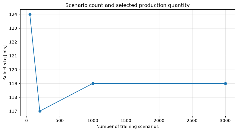
Scenario optimization generates $(D_s,Y_s)$ from historical data and predictive models, and applies the same $q$ to all scenarios. The plan selected for the training scenario is evaluated using separately generated validation scenarios to check for overfits.

Check with Python

train_sizes = [50, 200, 1000, 3000]
rows = []
for n in train_sizes:
    idx = rng.choice(n_scenarios, size=n, replace=False)
    train_scores = [profit(q, demand[idx], yield_rate[idx]).mean() for q in q_grid]
    q_hat = q_grid[np.argmax(train_scores)]
    rows.append([n, q_hat, profit(q_hat).mean(), (q_hat*yield_rate < demand).mean()])
stability_073 = pd.DataFrame(rows, columns=["scenario_count", "selected_q", "validation_profit", "validation_shortage_rate"])
display(stability_073.round(3))

fig, ax = plt.subplots()
ax.plot(stability_073["scenario_count"], stability_073["selected_q"], marker="o")
ax.set_title("Scenario count and selected production quantity")
ax.set_xlabel("Number of training scenarios")
ax.set_ylabel("Selected q [lots]")
ax.grid(True, alpha=.3)
plt.tight_layout()
plt.show()

	scenario_count	selected_q	validation_profit	validation_shortage_rate
0	50	124	68.695	0.206
1	200	117	68.926	0.318
2	1000	119	69.028	0.283
3	3000	119	69.028	0.283

Reading the results

If the number of scenarios is small, the recommended amount will be adjusted based on the demand mix that happens to be included. Select a number where the recommended amount and validation KPIs are sufficiently stable, and record the generation logic, random seed, and target period.

No.074: Chance Constraint

Meaning in Practice

For key customers, a service level is needed that is not “average enough,” but “at least 95% of the time demand is met.”

Approach to Analysis and Modeling

If the probability of allowing stockouts to be $\alpha$, the chance constraint is

$\Pr(qY\ge D)\ge 1-\alpha$

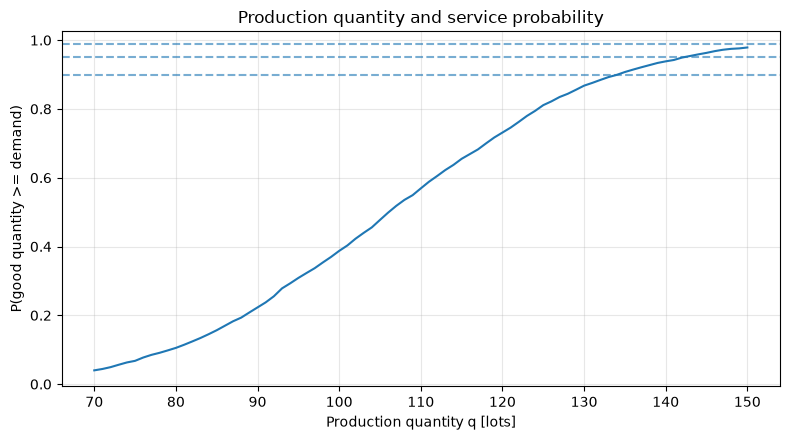
That’s right. Here, we approximate the fulfillment rate in the scenario and find the minimum production quantity that meets the constraints. Since estimation errors exist with finite samples, confidence intervals and safety margins are also considered in actual operation.

Check with Python

service = np.array([(q*yield_rate >= demand).mean() for q in q_grid])
chance_rows = []
for target in [.90, .95, .99]:
    feasible = q_grid[service >= target]
    q_req = int(feasible[0]) if len(feasible) else np.nan
    chance_rows.append([target, q_req, profit(q_req).mean() if np.isfinite(q_req) else np.nan])
chance_074 = pd.DataFrame(chance_rows, columns=["target_service", "minimum_q", "expected_profit"])
display(chance_074.round(2))

fig, ax = plt.subplots()
ax.plot(q_grid, service, label="Estimated service probability")
for target in [.90, .95, .99]: ax.axhline(target, linestyle="--", alpha=.6)
ax.set_title("Production quantity and service probability")
ax.set_xlabel("Production quantity q [lots]")
ax.set_ylabel("P(good quantity >= demand)")
ax.grid(True, alpha=.3)
plt.tight_layout()
plt.show()

	target_service	minimum_q	expected_profit
0	0.90	135.0	65.61
1	0.95	143.0	62.15
2	0.99	NaN	NaN

Reading the results

The higher the service target, the more the required amount increases nonlinearly. Rather than imposing a uniform 99%, set targets by comparing the impact of out-of-stock and additional costs by customer and part number.

No.075: Robust Optimization

Meaning in Practice

For new products or disaster response products where predicted distributions are difficult to trust, the likelihood of “protection anywhere within the expected range” may be prioritized over occurrence probability.

Approach to Analysis and Modeling

Constraints that can be fulfilled even under worst-case conditions from the demand ceiling $D^{U}$ and yield floor $Y^{L}$

$qY^{L}\ge D^{U}$

Place. While probability is not required, if the uncertainty set is too large, it leads to overproduction.

Check with Python

robust_rows = []
for d_upper, y_lower, label in [(125,.91,"moderate"),(140,.88,"strict"),(160,.84,"extreme")]:
    q_req = int(np.ceil(d_upper/y_lower))
    robust_rows.append([label,d_upper,y_lower,q_req,profit(q_req).mean(),(q_req*yield_rate>=demand).mean()])
robust_075 = pd.DataFrame(robust_rows, columns=["uncertainty_set","demand_upper","yield_lower","q","expected_profit","service_rate"])
display(robust_075.round(2))

	uncertainty_set	demand_upper	yield_lower	q	expected_profit	service_rate
0	moderate	125	0.91	138	64.40	0.93
1	strict	140	0.88	160	53.15	0.99
2	extreme	160	0.84	191	35.62	1.00

Reading the results

The more uncertain the set of uncertainties, the higher the service rate becomes, but the average profit can decline. We do not arbitrarily set upper or lower limits; instead, we agree on past forecast errors, equipment failure history, and BCP policies.

No.076: Distribution-Robust Optimization

Meaning in Practice

Stochastic programming depends on whether the estimated distribution is correct. If there are few samples or the composition changes with a new product, it is necessary to be prepared for deviations in the distribution itself.

Approach to Analysis and Modeling

Distributed Robust Optimization (DRO) evaluates the worst-case expected benefit among candidate distribution sets $\mathcal P$.

$\max_q\min_{P\in\mathcal P}\mathbb E_P[\pi(q,D,Y)]$

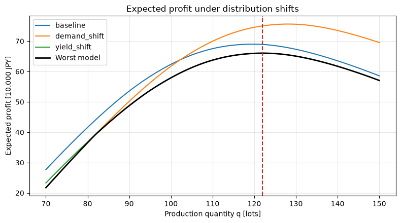
Here, for explanation, we create three distribution models: standard, demand fluctuations, and yield deterioration to maximize their minimum expected returns.

Check with Python

models = {
    "baseline": (demand, yield_rate),
    "demand_shift": (demand+8, yield_rate),
    "yield_shift": (demand, np.clip(yield_rate-.025,.80,1.0)),
}
model_profit = pd.DataFrame({name:[profit(q,d,y).mean() for q in q_grid] for name,(d,y) in models.items()}, index=q_grid)
worst_expected = model_profit.min(axis=1)
q_dro = int(worst_expected.idxmax())
display(pd.DataFrame({"model":model_profit.columns,"expected_profit_at_DRO":model_profit.loc[q_dro].values}).round(2))
print("DRORecommended production volume of wind:", q_dro, "  Worst-case model expected profit:", round(worst_expected.loc[q_dro],2))

fig, ax = plt.subplots()
for col in model_profit: ax.plot(q_grid, model_profit[col], label=col)
ax.plot(q_grid, worst_expected, color="black", linewidth=2, label="Worst model")
ax.axvline(q_dro, color="tab:red", linestyle="--")
ax.set_title("Expected profit under distribution shifts")
ax.set_xlabel("Production quantity q [lots]")
ax.set_ylabel("Expected profit [10,000 JPY]")
ax.grid(True, alpha=.3)
ax.legend()
plt.tight_layout()
plt.show()

	model	expected_profit_at_DRO
0	baseline	68.93
1	demand_shift	75.04
2	yield_shift	66.05

Recommended production volume for DRO wind: 122 Worst model expected profit: 66.05

Reading the results

DRO wind planning reduces reliance on a single estimated distribution. In practice, since the size of the distribution set determines maintainability, backtesting is conducted to verify “how much distribution deviation is covered.”

No.077: Multipurpose Optimization

Meaning in Practice

Manufacturing planning serves multiple purposes, including profit, delivery time, CO2, and overtime. If you can’t convert everything into monetary value, instead of deciding on a single answer first, compare candidates with different weights.

Approach to Analysis and Modeling

Assume the CO2 from regular production is 5.2 kg per lot, and the express response in case of out-of-stock is set at 11 kg per shortage lot, and the expected CO2 is calculated. Weighted Japanese

$\max_q\{\mathbb E[\pi(q)]-\lambda\mathbb E[C(q)]\}$

Change $\lambda$. It is important to clearly specify the unit and scale for the target value.

Check with Python

def expected_co2(q):
    shortage = np.maximum(demand-q*yield_rate,0)
    return 5.2*q + 11.0*shortage.mean()

co2 = np.array([expected_co2(q) for q in q_grid])
multi_rows=[]
for lam in [0, .02, .05, .10, .20]:
    score=expected_profit-lam*co2
    i=np.argmax(score)
    multi_rows.append([lam,q_grid[i],expected_profit[i],co2[i],service[i]])
multi_077=pd.DataFrame(multi_rows,columns=["carbon_weight","q","expected_profit","expected_co2","service_rate"])
display(multi_077.round(2))

	carbon_weight	q	expected_profit	expected_co2	service_rate
0	0.00	119	69.03	656.43	0.72
1	0.02	118	68.99	654.19	0.70
2	0.05	117	68.93	652.11	0.68
3	0.10	114	68.54	646.79	0.64
4	0.20	112	68.11	644.05	0.60

Reading the results

Changing the carbon weight affects the recommended amount and service rate. Weights are not set behind closed doors by analysts, but are linked to internal policies such as carbon pricing, customer requirements, and SBT.

No.078: Best for Pareto

Meaning in Practice

Candidates who can improve profits while reducing CO2 emissions are clearly inferior. If you only leave candidates whose improvement will worsen the other, you can narrow down the options necessary for management decisions.

Approach to Analysis and Modeling

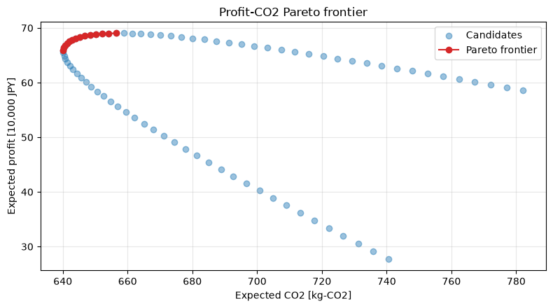
If candidate A has more profit than B and less CO2 than B, and at least one is strictly superior, A dominates B. Pareto is best because it is not dominated by any contender. The Pareto set is not the “only correct answer,” but a boundary for making value judgments.

Check with Python

pareto=[]
for i,q in enumerate(q_grid):
    dominated=np.any((expected_profit>=expected_profit[i]) & (co2<=co2[i]) & ((expected_profit>expected_profit[i]) | (co2<co2[i])))
    if not dominated: pareto.append(i)
pareto_078=pd.DataFrame({"q":q_grid[pareto],"expected_profit":expected_profit[pareto],"expected_co2":co2[pareto],"service_rate":service[pareto]})
display(pareto_078.iloc[::max(1,len(pareto_078)//8)].round(2))

fig, ax = plt.subplots()
ax.scatter(co2, expected_profit, alpha=.45, label="Candidates")
ax.plot(co2[pareto], expected_profit[pareto], color="tab:red", marker="o", label="Pareto frontier")
ax.set_title("Profit-CO2 Pareto frontier")
ax.set_xlabel("Expected CO2 [kg-CO2]")
ax.set_ylabel("Expected profit [10,000 JPY]")
ax.grid(True, alpha=.3)
ax.legend()
plt.tight_layout()
plt.show()

	q	expected_profit	expected_co2	service_rate
0	106	65.95	640.16	0.50
1	107	66.40	640.35	0.52
2	108	66.82	640.75	0.54
3	109	67.20	641.29	0.55
4	110	67.54	642.01	0.57
5	111	67.85	642.94	0.59
6	112	68.11	644.05	0.60
7	113	68.34	645.34	0.62
8	114	68.54	646.79	0.64
9	115	68.70	648.42	0.66
10	116	68.82	650.20	0.67
11	117	68.93	652.11	0.68
12	118	68.99	654.19	0.70
13	119	69.03	656.43	0.72

Reading the results

From the slope of the Pareto curve, you can read the CO2 increase for additional profit. In decision-making meetings, narrowing down to 3 to 5 representative proposals and presenting profit, CO2, and service rates in the same table makes it easier to reach consensus.

No.079: Risk Scales and CVaR

Meaning in Practice

Even if the average profit is the same, a plan that rarely runs a large deficit and a plan with stable losses are not the same. CVaR measures the average of the bad case group and represents downside risk to business continuity.

Approach to Analysis and Modeling

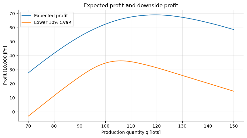
The bottom $\alpha$ percentile of profit is called $\mathrm{VaR}_{\alpha}$, and in this article, the average profit of the bottom $\alpha$ is referred to as the lower-tail CVaR.

$\mathrm{CVaR}^{\mathrm{profit}}_{\alpha}(q)=\mathbb E[\pi(q)\mid \pi(q)\le \mathrm{VaR}_{\alpha}(q)]$

The higher the price, the more profits are maintained even in bad cases. Note that the code is reversed from CVaR defined by loss.

Check with Python

alpha=.10
lower_cvar=[]
for q in q_grid:
    p=profit(q); threshold=np.quantile(p,alpha)
    lower_cvar.append(p[p<=threshold].mean())
lower_cvar=np.array(lower_cvar)

risk_rows=[]
for gamma in [0,.25,.5,.75,1.0]:
    score=(1-gamma)*expected_profit+gamma*lower_cvar
    i=np.argmax(score)
    risk_rows.append([gamma,q_grid[i],expected_profit[i],lower_cvar[i],service[i]])
risk_079=pd.DataFrame(risk_rows,columns=["risk_weight","q","expected_profit","lower_10pct_CVaR","service_rate"])
display(risk_079.round(2))

fig, ax = plt.subplots()
ax.plot(q_grid, expected_profit, label="Expected profit")
ax.plot(q_grid, lower_cvar, label="Lower 10% CVaR")
ax.set_title("Expected profit and downside profit")
ax.set_xlabel("Production quantity q [lots]")
ax.set_ylabel("Profit [10,000 JPY]")
ax.grid(True, alpha=.3)
ax.legend()
plt.tight_layout()
plt.show()

	risk_weight	q	expected_profit	lower_10pct_CVaR	service_rate
0	0.00	119	69.03	31.92	0.72
1	0.25	115	68.70	33.81	0.66
2	0.50	110	67.54	35.68	0.57
3	0.75	108	66.82	36.13	0.54
4	1.00	106	65.95	36.30	0.50

Reading the results

When risk weight increases, a plan is chosen to partially compromise average profit and improve lower-tier cases. The level and weight of CVaR are determined based on management losses such as financial capacity, penalties, and impact on key customers.

No.080: Production Planning Considering Demand Fluctuations

Meaning in Practice

Finally, we compare maximum expected profit, 95% service, robust, DRO style, and CVaR emphasis using the same KPIs. It is important not to choose based on the method name, but rather to select KPIs that align with your company’s scope of responsibility.

Approach to Analysis and Modeling

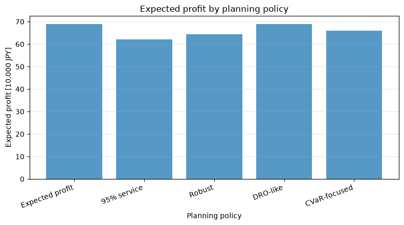
The $q$ determined by each policy are applied to common validation scenarios to evaluate expected profits, the bottom 10% CVaR, service rates, surplus volume, and CO2. In this article, we recommend that 95% of services are mandatory for key customers, with the plan where the expected profit is the highest.

Check with Python

q_chance=int(chance_074.loc[chance_074.target_service==.95,"minimum_q"].iloc[0])
q_robust=int(robust_075.loc[robust_075.uncertainty_set=="moderate","q"].iloc[0])
q_cvar=int(risk_079.loc[risk_079.risk_weight==1.0,"q"].iloc[0])
plans={"Expected profit":int(q_sto),"95% service":q_chance,"Robust":q_robust,"DRO-like":q_dro,"CVaR-focused":q_cvar}

rows=[]
for name,q in plans.items():
    p=profit(q); var=np.quantile(p,.10); good=q*yield_rate
    rows.append([name,q,p.mean(),p[p<=var].mean(),(good>=demand).mean(),np.maximum(good-demand,0).mean(),expected_co2(q)])
final_080=pd.DataFrame(rows,columns=["plan","q","expected_profit","lower_10pct_CVaR","service_rate","expected_surplus","expected_co2"])
display(final_080.round(2).sort_values("expected_profit",ascending=False))

eligible=final_080[final_080.service_rate>=.95]
recommended=eligible.loc[eligible.expected_profit.idxmax()]
print(f"Recommendation: {recommended['plan']} / q={int(recommended['q'])} lots")

fig, ax = plt.subplots()
x=np.arange(len(final_080))
ax.bar(x, final_080["expected_profit"], color="tab:blue", alpha=.75)
ax.set_xticks(x, final_080["plan"], rotation=20, ha="right")
ax.set_title("Expected profit by planning policy")
ax.set_xlabel("Planning policy")
ax.set_ylabel("Expected profit [10,000 JPY]")
ax.grid(True, axis="y", alpha=.3)
plt.tight_layout()
plt.show()

	plan	q	expected_profit	lower_10pct_CVaR	service_rate	expected_surplus	expected_co2
0	Expected profit	119	69.03	31.92	0.72	15.54	656.43
3	DRO-like	122	68.93	30.35	0.76	17.65	664.14
4	CVaR-focused	106	65.95	36.30	0.50	7.99	640.16
2	Robust	138	64.40	21.40	0.93	30.64	724.82
1	95% service	143	62.15	18.60	0.95	35.08	747.89

Recommended: 95% service / q=143 lots

Reading the results

Even with the same data, production volume and KPIs can vary depending on policy. In this example, 95% of the service was gated as a condition and recommended a plan with the highest expected profit within that constraint. In practice, candidate quantities are rounded down into equipment capacity, minimum lot, and setup units, and after rounding, all KPIs are re-evaluated.

Practical Implications Seen Through Target Exercise

• Average demand is a summary of inputs and does not leave the risk information necessary for decision-making.
• Probabilistic planning, chance constraints, robust optimization, and DRO differ from what you want to protect and the assumptions you want to protect.
• It is necessary not only to increase the number of scenarios but also to reflect the correlation between demand and yield, seasonality, and structural changes.
• Compare the additional costs of improving service rates with the losses caused by out-of-stock using the same meeting materials.
• In multipurpose questions, candidates for Pareto are presented, and the weight of the objective is treated as a management decision.
• CVaR visualizes bad cases that are not visible on average, but clearly defines target probabilities and signs.

What is necessary for practical implementation

1. Setting the boundaries of decision-making: Define the target part number, period, and the scope of normal production, outsourcing, and inventory.
2. Take stock of profit and loss: Not only manufacturing costs, but also stockouts, express shipping, disposal, overtime, and customer impact are organized.
3. Verify the scenario: Backtesting during unused periods, including forecast errors, correlations, busy periods, and equipment outages.
4. Agree on a risk policy: Service level, uncertainty set, and CVaR level are determined by sales, manufacturing, and finance.
5. Implement on-site constraints: Add capacity, scheduling, minimum lot, storage, raw materials, and personnel to the model.
6. Monitor operations: Stores recommended values, adoption values, reasons for overwriting, performance KPIs, and distribution deviations, and sets conditions for retraining.

Conclusion

In production planning under uncertainty, the starting point is to evaluate profits and services across multiple scenarios rather than focusing on a single forecast. Probabilistic planning focuses on average outcomes, chance constraints focus on the probability of achievement, robust optimization guarantees assumed ranges, DRO focuses on distribution deviation, and CVaR focuses on downside risk. Before choosing an optimization method, defining what and to what extent to be followed leads to an explainable and actionable plan.

Consultations for Corporations

At Suri Kobo, we support production and inventory planning, service level design, scenario generation, and building decision-making logic that integrates uncertainties in demand forecasts, including demand forecasting uncertainties. A PoC can start by comparing with current rules, designing KPIs, backtesting, and organizing on-site constraints.

📩 Contact Us: surikobo.co.jp/contact
Please feel free to consult us first.