Connecting Factory Decision-Making: 10 Exercises on Production, Scheduling, Inventory, and Investment Optimization

Using a fictional precision parts factory as the subject, it handles everything from monthly production volumes to daily work schedules, personnel, inventory, orders, and capital investment as consistent decision-making. The target is No.091〜No.100(ManufacturingDIApplication to.

Here, DI (Decision Intelligence) refers to a system that does not just look at forecasts but translates them under constraints into “what to do, when, and how much to execute,” improving next decisions based on actual results.

[!NOTE] This material is a notebook previously used by Surikoubo (or personally by the representative, Kazuyama), and has been reconstructed, edited, and published with the company’s permission.
All data listed is fictional and has no relation whatsoever to real companies, factories, or figures.

Introduction: Practical Challenges in Manufacturing Covered in This Article

Sales plans tend to be made by product, equipment plans by machine, personnel plans by skills, and procurement plans by components. However, on the ground, increasing production increases planning and overtime, reducing inventory raises the risk of stockouts, and purchasing equipment changes fixed costs and future options. In this article, we connect these together with common data and objective metrics.

Common situations on site

• Each Excel has different required requirements and capabilities.
• Departmental KPIs such as “delivery priority” and “minimum inventory” clash
• Practical constraints such as skilled personnel, planning, and maintenance stoppages are not reflected in the plan.
• Optimization results are limited to just one number, and you can’t explain alternatives or how they deteriorate.

Why is this issue so difficult to judge?

Decision variables are interdependent and include both integer and uncertainty. Because of forecasting errors, a plan that works out of the box may not always be executable as is. Therefore, it is necessary to clearly state objective functions, constraints, temporal granularity, and replanning conditions, and evaluate effectiveness by comparing with the current proposal.

Overview of Exercise covered this time

No.	Theme	Key Decisions	Key Evaluation Indicators
091	Production Planning Optimization	Production volume by product	Marginal Interests, Capacity Margin
092	job shop	Work Sequence by Equipment	makespan
093	Flow Shop	Common Input Order for All Processes	Completion time
094	Line balancing	Work process allocation	Cycle time, efficiency
095	staffing	Skill-based shifts	Adequacy Rate, Personnel Expenses
096	Inventory optimization	Safety Stock & Ordering Point	Service Rate, Holdings
097	Order volume optimization	lot size	Order cost + storage fee
098	Capital Investment Optimization	Portfolio of Investment Projects	NPV, budget consumption
099	Simulation × Optimization	Policy under uncertainty	Total cost distribution, out-of-stock rate
100	Decision Engine	From input to approval	Value, Feasibility, Auditability

Preparing the Python environment

No external data is used. Using only NumPy, pandas, SciPy, and Matplotlib, fix the random number generator’s seed and make it reproducible.

import platform
import itertools
import numpy as np
import pandas as pd
import matplotlib
import matplotlib.pyplot as plt
import scipy
from scipy.optimize import linprog
from IPython.display import display

rng = np.random.default_rng(42)
plt.rcParams.update({"figure.figsize": (8, 4), "axes.grid": True})
print(f"Python {platform.python_version()}")
print(f"NumPy {np.__version__} / pandas {pd.__version__} / SciPy {scipy.__version__} / Matplotlib {matplotlib.__version__}")

Python 3.13.1
NumPy 2.5.1 / pandas 3.0.3 / SciPy 1.18.0 / Matplotlib 3.11.0

Creation of Fictional Data

We envision a precision parts factory with three products, multiple equipment, skilled personnel, and key components. The unit of amount is thousand yen, the hour unit is time, and the unit of demand and inventory is pieces. Derive the detailed data required for each analysis from this master.

products = pd.DataFrame({
    "product": ["A-Standard", "B-High Precision", "C-Short delivery time"],
    "demand": [420, 300, 260], "contribution": [8.0, 11.0, 9.0],
    "machining_h": [1.0, 1.6, 1.2], "assembly_h": [0.8, 0.7, 1.1],
    "material_kg": [2.0, 2.8, 1.7]
})
capacity = pd.Series({"machining_h": 1150, "assembly_h": 850, "material_kg": 2200})
jobs = pd.DataFrame({"job": list("ABCDEF"), "M1": [4, 7, 3, 6, 5, 4],
                     "M2": [6, 3, 5, 4, 7, 2], "M3": [3, 5, 4, 6, 2, 5]})
display(products)
display(capacity.rename("monthly_capacity").to_frame())
display(jobs)

	product	demand	contribution	machining_h	assembly_h	material_kg
0	A-Standard	420	8.0	1.0	0.8	2.0
1	B-High Precision	300	11.0	1.6	0.7	2.8
2	C-Short delivery time	260	9.0	1.2	1.1	1.7

	monthly_capacity
machining_h	1150
assembly_h	850
material_kg	2200

	job	M1	M2	M3
0	A	4	6	3
1	B	7	3	5
2	C	3	5	4
3	D	6	4	6
4	E	5	7	2
5	F	4	2	5

No.091: Production Planning Optimization

Meaning in Practice

Within the upper limit of demand, it decides which products to allocate limited processing, assembly, and materials. The key issue is not “high-sales products,” but rather what to use one hour of bottleneck capability for to contribute to profit.

Approach to Analysis and Modeling

If we $x_i$ the production volume of product $i$, $p_i$ marginal profit, and $a_{ri}$ resource usage,

$\max_x \sum_i p_i x_i \quad \text{s.t.}\quad \sum_i a_{ri}x_i\le C_r,\;0\le x_i\le d_i$

It can be expressed as such. Here, continuous solutions of linear programming are set as monthly goals, and in actual operation, constraints are rounded down to lot-level units and then re-examined.

Check with Python

resource_cols = ["machining_h", "assembly_h", "material_kg"]
r91 = linprog(-products["contribution"], A_ub=products[resource_cols].to_numpy().T,
              b_ub=capacity.to_numpy(), bounds=list(zip(np.zeros(3), products["demand"])), method="highs")
plan = products[["product", "demand"]].copy()
plan["optimal_qty"] = r91.x
plan["contribution_kJPY"] = r91.x * products["contribution"]
usage = pd.DataFrame({"capacity": capacity, "used": products[resource_cols].to_numpy().T @ r91.x})
usage["utilization_%"] = 100 * usage["used"] / usage["capacity"]
display(plan.round(1)); display(usage.round(1))
ax = plan.set_index("product")[["demand", "optimal_qty"]].plot.bar()
ax.set(title="Demand and optimized production plan", xlabel="Product", ylabel="Quantity")
ax.grid(axis="y"); plt.tight_layout(); plt.show()

	product	demand	optimal_qty	contribution_kJPY
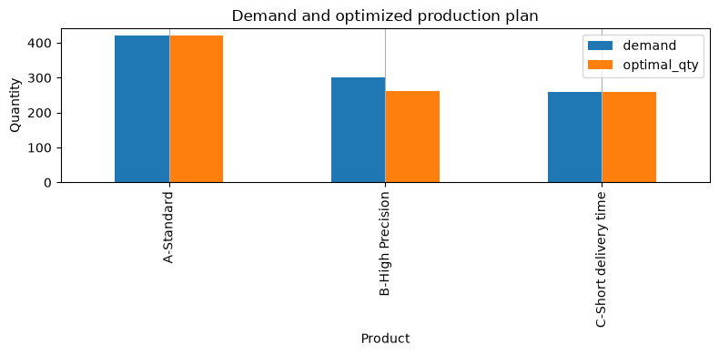
0	A-Standard	420	420.0	3360.0
1	B-High Precision	300	261.2	2873.8
2	C-Short delivery time	260	260.0	2340.0

	capacity	used	utilization_%
machining_h	1150	1150.0	100.0
assembly_h	850	804.9	94.7
material_kg	2200	2013.5	91.5

/var/folders/3y/fmw40k0x78xblvb3gkcyvy1h0000gn/T/ipykernel_11861/2709310365.py:12: UserWarning: Glyph 27161 (\N{CJK UNIFIED IDEOGRAPH-6A19}) missing from font(s) DejaVu Sans.
  ax.grid(axis="y"); plt.tight_layout(); plt.show()
/var/folders/3y/fmw40k0x78xblvb3gkcyvy1h0000gn/T/ipykernel_11861/2709310365.py:12: UserWarning: Glyph 28310 (\N{CJK UNIFIED IDEOGRAPH-6E96}) missing from font(s) DejaVu Sans.
  ax.grid(axis="y"); plt.tight_layout(); plt.show()
/var/folders/3y/fmw40k0x78xblvb3gkcyvy1h0000gn/T/ipykernel_11861/2709310365.py:12: UserWarning: Glyph 39640 (\N{CJK UNIFIED IDEOGRAPH-9AD8}) missing from font(s) DejaVu Sans.
  ax.grid(axis="y"); plt.tight_layout(); plt.show()
/var/folders/3y/fmw40k0x78xblvb3gkcyvy1h0000gn/T/ipykernel_11861/2709310365.py:12: UserWarning: Glyph 31934 (\N{CJK UNIFIED IDEOGRAPH-7CBE}) missing from font(s) DejaVu Sans.
  ax.grid(axis="y"); plt.tight_layout(); plt.show()
/var/folders/3y/fmw40k0x78xblvb3gkcyvy1h0000gn/T/ipykernel_11861/2709310365.py:12: UserWarning: Glyph 24230 (\N{CJK UNIFIED IDEOGRAPH-5EA6}) missing from font(s) DejaVu Sans.
  ax.grid(axis="y"); plt.tight_layout(); plt.show()
/var/folders/3y/fmw40k0x78xblvb3gkcyvy1h0000gn/T/ipykernel_11861/2709310365.py:12: UserWarning: Glyph 30701 (\N{CJK UNIFIED IDEOGRAPH-77ED}) missing from font(s) DejaVu Sans.
  ax.grid(axis="y"); plt.tight_layout(); plt.show()
/var/folders/3y/fmw40k0x78xblvb3gkcyvy1h0000gn/T/ipykernel_11861/2709310365.py:12: UserWarning: Glyph 32013 (\N{CJK UNIFIED IDEOGRAPH-7D0D}) missing from font(s) DejaVu Sans.
  ax.grid(axis="y"); plt.tight_layout(); plt.show()
/var/folders/3y/fmw40k0x78xblvb3gkcyvy1h0000gn/T/ipykernel_11861/2709310365.py:12: UserWarning: Glyph 26399 (\N{CJK UNIFIED IDEOGRAPH-671F}) missing from font(s) DejaVu Sans.
  ax.grid(axis="y"); plt.tight_layout(); plt.show()
/Users/hiroshi/private/kobo/notebook/.venv/lib/python3.13/site-packages/IPython/core/pylabtools.py:170: UserWarning: Glyph 27161 (\N{CJK UNIFIED IDEOGRAPH-6A19}) missing from font(s) DejaVu Sans.
  fig.canvas.print_figure(bytes_io, **kw)
/Users/hiroshi/private/kobo/notebook/.venv/lib/python3.13/site-packages/IPython/core/pylabtools.py:170: UserWarning: Glyph 28310 (\N{CJK UNIFIED IDEOGRAPH-6E96}) missing from font(s) DejaVu Sans.
  fig.canvas.print_figure(bytes_io, **kw)
/Users/hiroshi/private/kobo/notebook/.venv/lib/python3.13/site-packages/IPython/core/pylabtools.py:170: UserWarning: Glyph 39640 (\N{CJK UNIFIED IDEOGRAPH-9AD8}) missing from font(s) DejaVu Sans.
  fig.canvas.print_figure(bytes_io, **kw)
/Users/hiroshi/private/kobo/notebook/.venv/lib/python3.13/site-packages/IPython/core/pylabtools.py:170: UserWarning: Glyph 31934 (\N{CJK UNIFIED IDEOGRAPH-7CBE}) missing from font(s) DejaVu Sans.
  fig.canvas.print_figure(bytes_io, **kw)
/Users/hiroshi/private/kobo/notebook/.venv/lib/python3.13/site-packages/IPython/core/pylabtools.py:170: UserWarning: Glyph 24230 (\N{CJK UNIFIED IDEOGRAPH-5EA6}) missing from font(s) DejaVu Sans.
  fig.canvas.print_figure(bytes_io, **kw)
/Users/hiroshi/private/kobo/notebook/.venv/lib/python3.13/site-packages/IPython/core/pylabtools.py:170: UserWarning: Glyph 30701 (\N{CJK UNIFIED IDEOGRAPH-77ED}) missing from font(s) DejaVu Sans.
  fig.canvas.print_figure(bytes_io, **kw)
/Users/hiroshi/private/kobo/notebook/.venv/lib/python3.13/site-packages/IPython/core/pylabtools.py:170: UserWarning: Glyph 32013 (\N{CJK UNIFIED IDEOGRAPH-7D0D}) missing from font(s) DejaVu Sans.
  fig.canvas.print_figure(bytes_io, **kw)
/Users/hiroshi/private/kobo/notebook/.venv/lib/python3.13/site-packages/IPython/core/pylabtools.py:170: UserWarning: Glyph 26399 (\N{CJK UNIFIED IDEOGRAPH-671F}) missing from font(s) DejaVu Sans.
  fig.canvas.print_figure(bytes_io, **kw)

Reading the results

Rather than meeting all demand, constrained resources are allocated to combinations with higher profit contributions. Resources with an operating rate close to 100% are bottlenecks for increased production. However, rounding fractions into lots can result in exceedance, so re-verification after rounding and minimum supply constraints are necessary.

No.092: Job Shop Scheduling

Meaning in Practice

In processing sites where the equipment sequence passes through different jobs for each job, it is necessary to plan to ensure that work does not overlap with the same equipment and to follow the process order for each job. It affects not only delivery delays but also work-on backlogs and rescheduling.

Approach to Analysis and Modeling

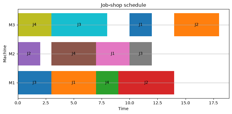
Set the start time of work $(j,k)$ as $s_{jk}$, impose process lead constraints and non-duplication constraints on equipment, and minimize the $C_{\max}$ of total task completion times. Here, we solve small-scale examples using dispatch rules that prioritize tasks that can be executed early. It is also important to note that it is not always strictly optimal.

Check with Python

routes = {
 "J1": [("M1",4),("M2",3),("M3",2)], "J2": [("M2",2),("M1",5),("M3",4)],
 "J3": [("M1",3),("M3",5),("M2",2)], "J4": [("M3",3),("M2",4),("M1",2)]}
machine_free = {m: 0 for m in ["M1","M2","M3"]}; job_free = {j: 0 for j in routes}; sched=[]
remaining = [(j,k,m,p) for j,ops in routes.items() for k,(m,p) in enumerate(ops)]
while remaining:
    eligible = [x for x in remaining if x[1] == sum(1 for r in sched if r[0] == x[0])]
    j,k,m,p = min(eligible, key=lambda x:(max(job_free[x[0]],machine_free[x[2]]), x[3]))
    start=max(job_free[j],machine_free[m]); end=start+p
    sched.append((j,k,m,start,end)); job_free[j]=end; machine_free[m]=end; remaining.remove((j,k,m,p))
sched_df=pd.DataFrame(sched,columns=["job","operation","machine","start","end"])
display(sched_df.sort_values(["machine","start"]))
fig,ax=plt.subplots()
for y,(m,g) in enumerate(sched_df.groupby("machine")):
    for _,r in g.iterrows(): ax.barh(y,r.end-r.start,left=r.start); ax.text((r.start+r.end)/2,y,r.job,ha="center",va="center")
ax.set_yticks(range(3), sorted(sched_df.machine.unique())); ax.set(title="Job-shop schedule",xlabel="Time",ylabel="Machine")
ax.grid(axis="x"); plt.tight_layout(); plt.show()
print("Makespan:", sched_df.end.max())

	job	operation	machine	start	end
1	J3	0	M1	0	3
3	J1	0	M1	3	7
6	J4	2	M1	7	9
8	J2	1	M1	9	14
0	J2	0	M2	0	2
4	J4	1	M2	3	7
7	J1	1	M2	7	10
10	J3	2	M2	10	12
2	J4	0	M3	0	3
5	J3	1	M3	3	8
9	J1	2	M3	10	12
11	J2	2	M3	14	18

Makespan: 18

Reading the results

There are no duplicates in the Gantt diagram, and the order of each job is followed. On the other hand, equipment gaps also occur while waiting for the previous process. In practice, we compare current rules, including deadlines, priorities, setup queues, and downtime, as well as makeup span, delays, and stability.

No.093: Flow Shop Scheduling

Meaning in Practice

On a line where all products follow the same process sequence, even just the order of input can greatly affect the waiting time for subsequent processes. If you simply change the order, there is a possibility of improving without capital investment.

Approach to Analysis and Modeling

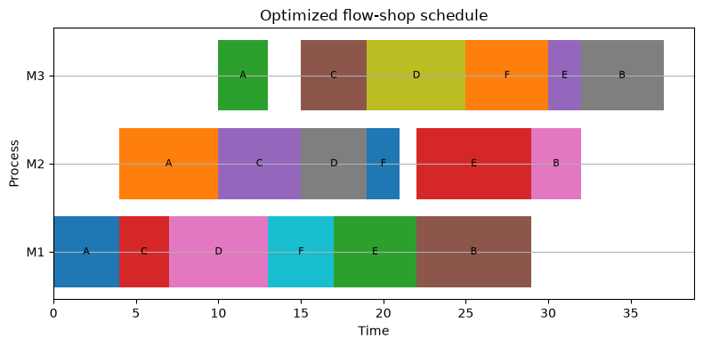
For permutation $\pi$, the completion time can be recursively calculated in $C_{k,m}=\max(C_{k-1,m},C_{k,m-1})+p_{\pi_k,m}$. Since there are 6 jobs, you list all $6!=720$ permutations and find the minimum makespan.

Check with Python

def flow_completion(order):
    c=np.zeros((len(order),3))
    for i,j in enumerate(order):
        for m,col in enumerate(["M1","M2","M3"]):
            c[i,m]=max(c[i-1,m] if i else 0,c[i,m-1] if m else 0)+jobs.set_index("job").loc[j,col]
    return c
records=[]
for order in itertools.permutations(jobs.job): records.append((order,flow_completion(order)[-1,-1]))
records.sort(key=lambda x:x[1]); best_order,best_ms=records[0]; base=tuple(jobs.job); base_ms=flow_completion(base)[-1,-1]
display(pd.DataFrame({"plan":["Current","Optimized"],"order":["→".join(base),"→".join(best_order)],"makespan":[base_ms,best_ms]}))
c=flow_completion(best_order); fig,ax=plt.subplots()
for i,j in enumerate(best_order):
 for m in range(3):
  p=jobs.set_index("job").loc[j,f"M{m+1}"]; ax.barh(m,p,left=c[i,m]-p); ax.text(c[i,m]-p/2,m,j,ha="center",va="center",fontsize=8)
ax.set_yticks(range(3),["M1","M2","M3"]); ax.set(title="Optimized flow-shop schedule",xlabel="Time",ylabel="Process")
ax.grid(axis="x"); plt.tight_layout(); plt.show()

	plan	order	makespan
0	Current	A→B→C→D→E→F	39.0
1	Optimized	A→C→D→F→E→B	37.0

Reading the results

The gap in makeup span between the current and best order is an area for improvement when changing the order of deployment. If there are multiple permutations with the best tie, you can select delivery time and setup stability as secondary indicators. As the number of varieties increases, the total enumeration surges, so switch to integer planning or heuristics.

No.094: Line Balancing

Meaning in Practice

Assembly work is assigned to the process, reducing load differences between processes while maintaining tact. Since the maximum load process determines the overall production speed of the line, it is not possible to judge based solely on average time.

Approach to Analysis and Modeling

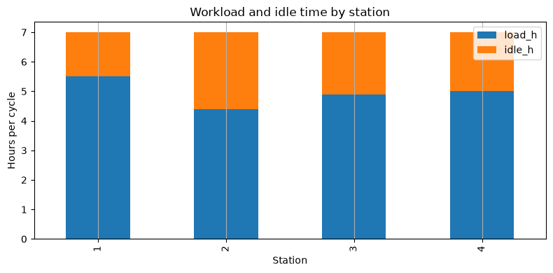
If the total work time is $T$, the number of processes is $K$, and cycle time is $C$, the line efficiency is $E=T/(KC)$. Idle time is allocated using a simple position-weighting method that protects the prior relationship.

Check with Python

tasks=pd.DataFrame({"task":list("ABCDEFGH"),"time":[2.4,3.1,1.8,2.6,3.4,1.5,2.2,2.8]})
cycle=7.0; stations=[]; current=[]; load=0
for _,r in tasks.iterrows():
    if load+r.time>cycle: stations.append((current,load)); current=[]; load=0
    current.append(r.task); load+=r.time
stations.append((current,load))
bal=pd.DataFrame({"station":range(1,len(stations)+1),"tasks":[",".join(s[0]) for s in stations],"load_h":[s[1] for s in stations]})
bal["idle_h"]=cycle-bal.load_h; efficiency=tasks.time.sum()/(len(bal)*cycle)
display(bal.round(1)); print(f"Line efficiency: {efficiency:.1%}")
ax=bal.plot.bar(x="station",y=["load_h","idle_h"],stacked=True)
ax.set(title="Workload and idle time by station",xlabel="Station",ylabel="Hours per cycle"); ax.grid(axis="y"); plt.tight_layout(); plt.show()

	station	tasks	load_h	idle_h
0	1	A,B	5.5	1.5
1	2	C,D	4.4	2.6
2	3	E,F	4.9	2.1
3	4	G,H	5.0	2.0

Line efficiency: 70.7%

Reading the results

Rather than blaming only low-load processes, we check prior relationships, whether work can be split, and limitations of skills and jigs. Since shortening cycle times gradually increases the number of required processes, personnel and efficiency are evaluated according to demand scenarios.

No.095: Personnel Allocation Optimization

Meaning in Practice

While meeting the daily required number of people, we decide on work patterns and personnel costs. Not only the number of people, but also skills, qualifications, continuous working hours, desired leave, and fairness all determine feasibility.

Approach to Analysis and Modeling

$a_{dp}$ $x_p$ the number of employees to be hired for work pattern $p$ and whether it covers the $d$ of days, we will denote $\min\sum_p c_px_p$ and $\sum_p a_{dp}x_p\ge r_d$. List the short-term integer candidates.

Check with Python

days=["Mon","Tue","Wed","Thu","Fri","Sat","Sun"]
patterns={"Weekday":[1,1,1,1,1,0,0],"Early":[1,1,1,0,0,1,1],"Late":[0,0,1,1,1,1,1],"Weekend":[0,0,0,0,0,1,1]}
required=np.array([6,7,8,8,7,5,4]); costs=np.array([210,205,215,90])
A=np.array(list(patterns.values())).T; candidates=[]
for x in itertools.product(range(10),repeat=4):
    cov=A@x
    if np.all(cov>=required): candidates.append((costs@x,*x,*cov))
best=min(candidates); staffing_cost=best[0]; x=np.array(best[1:5]); coverage=A@x
display(pd.DataFrame({"pattern":list(patterns),"staff":x,"weekly_cost_kJPY":x*costs}))
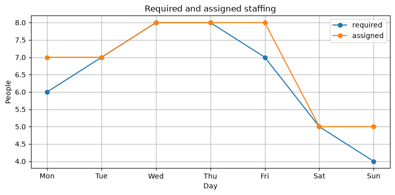
display(pd.DataFrame({"day":days,"required":required,"assigned":coverage,"surplus":coverage-required}))
ax=pd.DataFrame({"required":required,"assigned":coverage},index=days).plot(marker="o")
ax.set(title="Required and assigned staffing",xlabel="Day",ylabel="People"); ax.grid(True); plt.tight_layout(); plt.show()

	pattern	staff	weekly_cost_kJPY
0	Weekday	7	1470
1	Early	0	0
2	Late	1	215
3	Weekend	4	360

	day	required	assigned	surplus
0	Mon	6	7	1
1	Tue	7	7	0
2	Wed	8	8	0
3	Thu	8	8	0
4	Fri	7	8	1
5	Sat	5	5	0
6	Sun	4	5	1

Reading the results

This is a pattern configuration that meets the minimum cost required for a full day. Surplus is a side effect of integer work patterns and can be used for education and maintenance support. In actual operations, before directly optimizing individual names, labor regulations, qualifications for substitutability, fairness agreements, and accountability are established.

No.096: Inventory Optimization

Meaning in Practice

Inventory prevents stockouts while consuming funds, storage space, and the risk of obsolescence. It determines not only average demand but also safety stock for demand fluctuations during lead times.

Approach to Analysis and Modeling

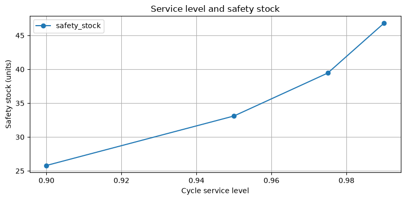
If daily demand is independent with an average of $\mu_d$, standard deviation $\sigma_d$, and lead time of $L$ days, the order point is $ROP=\mu_dL+z\sigma_d\sqrt{L}$. $z$ corresponds to the target cycle service rate.

Check with Python

mu_d,sigma_d,L=40,9,5
service_table=pd.DataFrame({"service_level":[0.90,0.95,0.975,0.99],"z":[1.282,1.645,1.960,2.326]})
service_table["safety_stock"]=service_table.z*sigma_d*np.sqrt(L)
service_table["reorder_point"]=mu_d*L+service_table.safety_stock
display(service_table.round(1))
ax=service_table.plot(x="service_level",y="safety_stock",marker="o")
ax.set(title="Service level and safety stock",xlabel="Cycle service level",ylabel="Safety stock (units)"); ax.grid(True); plt.tight_layout(); plt.show()

	service_level	z	safety_stock	reorder_point
0	0.9	1.3	25.8	225.8
1	1.0	1.6	33.1	233.1
2	1.0	2.0	39.4	239.4
3	1.0	2.3	46.8	246.8

Reading the results

The higher the service rate, the more nonlinear the safety stock increases. The choice is not about “higher is better,” but about comparing the impact of a single out-of-stock item with inventory costs. If there are significant differences in demand autocorrelation, lead time fluctuations, or carryover or lost orders during out-of-stock situations, we verify them through simulation rather than simple formulas.

No.097: Order Volume Optimization

Meaning in Practice

Small orders reduce average inventory but increase the number of orders, acceptances, and inspections. Bulk orders are the opposite. From this trade-off, the base lot is determined.

Approach to Analysis and Modeling

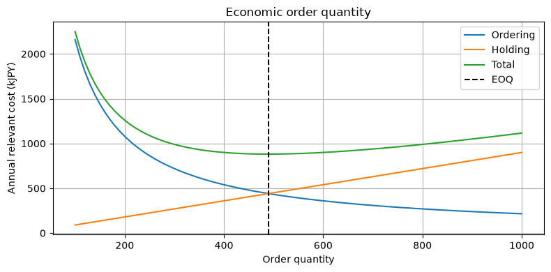
The economic order volume $D$ annual demand , $S$ per order cost, and $H$ annual storage cost per unit is $Q^*=\sqrt{2DS/H}$. The total related cost is $DS/Q+HQ/2$.

Check with Python

D,S,H=12000,18,1.8
q_star=np.sqrt(2*D*S/H); q=np.arange(100,1001,10)
ordering=D/q*S; holding=q/2*H; total=ordering+holding
print(f"EOQ: {q_star:.0f} units / relevant annual cost: {D/q_star*S+q_star/2*H:.1f} kJPY")
fig,ax=plt.subplots(); ax.plot(q,ordering,label="Ordering"); ax.plot(q,holding,label="Holding"); ax.plot(q,total,label="Total"); ax.axvline(q_star,color="black",ls="--",label="EOQ")
ax.set(title="Economic order quantity",xlabel="Order quantity",ylabel="Annual relevant cost (kJPY)"); ax.grid(True); ax.legend(); plt.tight_layout(); plt.show()

EOQ: 490 units / relevant annual cost: 881.8 kJPY

Reading the results

The total cost curve is relatively flat near the optimal point. Therefore, instead of using EOQ as an absolute value, you can compare nearby candidates by packaging unit, minimum order quantity, onboard efficiency, and storage ceiling. If there is a quantity discount, the price will be evaluated by price boundary, including the purchase cost.

No.098: Capital Investment Optimization

Meaning in Practice

Within the budget, select projects such as capacity enhancement, automated inspection, energy saving, and transport improvements. The payback years of individual projects alone cannot handle budget conflicts or set effects.

Approach to Analysis and Modeling

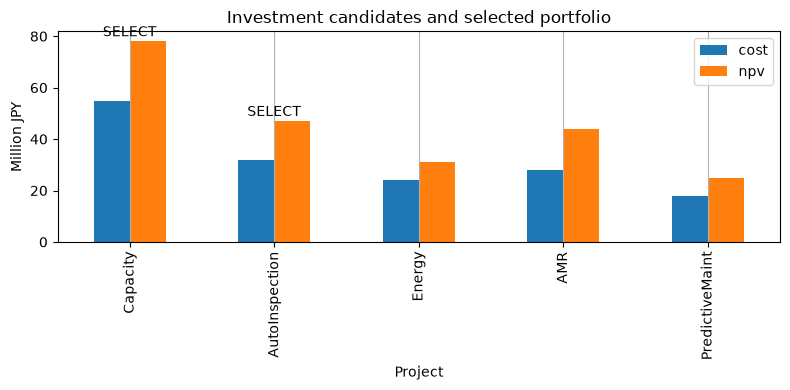
$y_i\in\{0,1\}$ the acceptance or rejection of Project $i$, the investment amount is set as $c_i$, NPV as $v_i$, and $\max\sum_i v_iy_i$ and $\sum_i c_iy_i\le B$. Furthermore, a dependency constraint of “automatic transport only when capacity enhancement is adopted” is applied to evaluate all combinations.

Check with Python

invest=pd.DataFrame({"project":["Capacity","AutoInspection","Energy","AMR","PredictiveMaint"],
 "cost":[55,32,24,28,18],"npv":[78,47,31,44,25]})
budget=90; opts=[]
for y in itertools.product([0,1],repeat=len(invest)):
    y=np.array(y); cost=y@invest.cost; value=y@invest.npv
    if cost<=budget and y[3]<=y[0]: opts.append((value,cost,y))
value,cost,y=max(opts,key=lambda z:z[0])
result=invest.copy(); result["selected"]=y.astype(bool); display(result); print(f"Total cost: {cost} / Budget: {budget} / Total NPV: {value}")
ax=result.plot.bar(x="project",y=["cost","npv"]); ax.set(title="Investment candidates and selected portfolio",xlabel="Project",ylabel="Million JPY");
for i,v in enumerate(y):
    if v: ax.text(i,max(result.loc[i,["cost","npv"]])+2,"SELECT",ha="center")
ax.grid(axis="y"); plt.tight_layout(); plt.show()

	project	cost	npv	selected
0	Capacity	55	78	True
1	AutoInspection	32	47	True
2	Energy	24	31	False
3	AMR	28	44	False
4	PredictiveMaint	18	25	False

Total cost: 87 / Budget: 90 / Total NPV: 125

Reading the results

The selection results simultaneously meet budget and dependencies. We check not only NPV point estimation but also whether rankings change in scenarios such as decreased demand, launch delays, and residual value. Even if there is an unspent budget, it is not necessarily abnormal because it is a discrete project.

No.099: Integration of Simulation and Optimization

Meaning in Practice

Optimal inventory policies based on average demand can frequently cause stockouts under fluctuating conditions. Candidate policies are compared across many identical demand scenarios and selected from both cost and service perspectives.

Approach to Analysis and Modeling

Candidate order points $r$ and order quantities $Q$ are selected, and daily inventory is simulated in Monte Carlo. The objective is average storage cost + order cost + out-of-stock penalty. Common random numbers are used to suppress comparison noise between candidates.

Check with Python

scenarios=rng.poisson(40,size=(120,180)); lead=5
def inventory_policy(r,Q):
    costs=[]; stockout_days=[]
    for demand_path in scenarios:
        onhand=r+Q; arrivals={}; cost=0; so=0
        for day,d in enumerate(demand_path):
            onhand+=arrivals.get(day,0); sold=min(onhand,d); lost=d-sold; onhand-=sold; so+=lost>0
            cost+=.003*onhand+.12*lost
            pipeline=sum(v for k,v in arrivals.items() if k>day)
            if onhand+pipeline<=r: arrivals[day+lead]=arrivals.get(day+lead,0)+Q; cost+=18
        costs.append(cost); stockout_days.append(so/len(demand_path))
    return np.mean(costs),np.quantile(costs,.95),np.mean(stockout_days)
rows=[]
for r in [180,200,220,240,260]:
 for Q in [300,450,600,750]: rows.append((r,Q,*inventory_policy(r,Q)))
policies=pd.DataFrame(rows,columns=["reorder_point","order_qty","mean_cost","p95_cost","stockout_day_rate"])
best=policies.loc[policies.mean_cost.idxmin()]; display(policies.sort_values("mean_cost").head(8).round(3))
pivot=policies.pivot(index="reorder_point",columns="order_qty",values="mean_cost")
fig,ax=plt.subplots(); im=ax.imshow(pivot,aspect="auto",origin="lower"); fig.colorbar(im,ax=ax,label="Mean cost")
ax.set_xticks(range(len(pivot.columns)),pivot.columns); ax.set_yticks(range(len(pivot.index)),pivot.index)
ax.set(title="Simulated policy cost",xlabel="Order quantity",ylabel="Reorder point"); ax.grid(False); plt.tight_layout(); plt.show()

	reorder_point	order_qty	mean_cost	p95_cost	stockout_day_rate
2	180	600	372.401	387.116	0.029
3	180	750	373.321	377.966	0.023
7	200	750	377.349	381.652	0.007
6	200	600	378.014	388.077	0.008
11	220	750	386.794	390.855	0.001
10	220	600	387.471	397.669	0.001
15	240	750	397.487	401.655	0.000
14	240	600	398.173	408.469	0.000

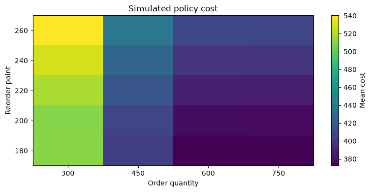
Reading the results

The top of the table shows the minimum average cost policy within the candidate set. However, if the average cost is close, there is room to choose options with 95% cost or shorter item rates. Simulation optimization stores random seed numbers, number of trials, comparison of identical scenarios with current policies, and inexperienced external validation periods.

No.100: Surikou’s Decision-Making Engine

Meaning in Practice

Value is not created by algorithms alone; it only emerges through a cycle of data acquisition, candidate generation, constraint validation, approval, execution, and performance learning. We will create a system where people can identify exceptions and track the reasons for recommendations.

Approach to Analysis and Modeling

Design the decision engine as a closed loop for Observe → Predict → Optimize → Simulate → Approve → Execute → Learn. Recommendations consolidate not only benefits but also constraint violations, risks, differences from current proposals, and reasons for adoption or rejection into one record.

Check with Python

decision_record=pd.DataFrame([
 ["Production plan",-r91.fun,"All resource use <= capacity","Approve if rounded plan remains feasible"],
 ["Staffing",-staffing_cost,"Assigned >= required","Supervisor reviews skills"],
 ["Inventory policy",-float(policies.mean_cost.min()),"Stockout-day rate monitored","Approve after shadow operation"],
 ["Investment portfolio",value,"Cost <= budget; dependencies","Board approves scenario assumptions"]],
 columns=["decision","objective_or_value","guardrail","human_gate"])
decision_record["run_id"]="DI-2026-07-001"; decision_record["data_version"]="synthetic-v1"
display(decision_record)
stages=pd.DataFrame({"stage":["Observe","Predict","Optimize","Simulate","Approve","Execute","Learn"],
                     "owner":["Data","Planning","OR","Risk","Manager","Operations","Analytics"]})
fig,ax=plt.subplots(figsize=(10,2.5)); ax.scatter(range(len(stages)),np.zeros(len(stages)),s=900)
for i,r in stages.iterrows(): ax.text(i,0,f"{r.stage}\n({r.owner})",ha="center",va="center",fontsize=8)
ax.plot(range(len(stages)),np.zeros(len(stages))); ax.set(title="Decision Intelligence operating loop",xlabel="Stage",ylabel="Workflow"); ax.set_yticks([]); ax.grid(axis="x"); plt.tight_layout(); plt.show()

	decision	objective_or_value	guardrail	human_gate	run_id	data_version
0	Production plan	8573.7500	All resource use <= capacity	Approve if rounded plan remains feasible	DI-2026-07-001	synthetic-v1
1	Staffing	-2045.0000	Assigned >= required	Supervisor reviews skills	DI-2026-07-001	synthetic-v1
2	Inventory policy	-372.4009	Stockout-day rate monitored	Approve after shadow operation	DI-2026-07-001	synthetic-v1
3	Investment portfolio	125.0000	Cost <= budget; dependencies	Board approves scenario assumptions	DI-2026-07-001	synthetic-v1

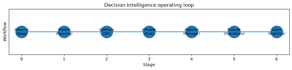
Reading the results

With the same run_id, you can track input versions, target values, guardrails, and human approval points. Rather than automation that eliminates people, it is designed to shift routine calculations to machines, where people take on exceptions, value judgments, and accountability. KPIs include not only the “target value for optimization,” but also proposal adoption rate, amount of manual revisions, replanning time, and performance differences.

Practical Implications Seen Through Target Exercise

• Production, schedules, personnel, inventory, and investment need to be connected by a common demand assumption and capability master.
• Before the optimal value, agree on the unit of the objective function, the absolute constraints to be observed, and the desired conditions.
• Showing differences from current proposals, alternatives, sensitivity, and constraint margins makes it easier for the field to make judgments.
• The impact of forecasting errors on decision-making is examined through scenarios or simulations.
• Manual revisions to recommended proposals are not failures but important logs for discovering unmodeled constraints.

What is necessary for practical implementation

Points of Contention	confirmation item	deliverable
Business Definition	Who decides, when, and what	Decision Flow, RACI
Data	Alignment of demand, capabilities, BOM, inventory, and skills at the time	Data Dictionary, Quality Reports
Mathematical model	Purpose, constraints, granularity, calculation time	Model Specifications and Test Cases
verification	Comparison with current proposals, past performance, and stress conditions	Effectiveness Verification and Sensitivity Analysis
Utilization	Replanning conditions, approvals, and alternative procedures in case of failure	Operational procedures and monitoring metrics
control	Tracking input versions, recommendations, corrections, and approvals	Audit Logs and Change Management

Implementation starts with small decisions, then uses shadow operations to compare with human plans, fixes loopholes in constraints, and then expands the scope of application.

Conclusion

From No.091 to No.100, individual optimizations were integrated into the manufacturing decision-making loop. A good model is not a complex one, but one that meets the constraints of the field, explains the reasons for results, and can be updated based on actual experience. It is practical to start by reproducing current decisions targeting one factory, one meeting body, and one KPI.

Consultations for Corporations

At Suri Kobo, we offer consultations on production planning, scheduling, inventory and ordering, staffing, capital investment, including problem organization, PoC, model development, integration with existing systems, and support for in-house production.

📩 Contact Us: surikobo.co.jp/contact
Please feel free to consult us first.