Protecting quality and equipment constraints simultaneously: 10 exercises to determine molding conditions explainably through convex optimization

Using a fictional resin molding process as the subject, you will learn about quality loss, power load, and equipment capacity using the same model to learn Conditions design that can explain to the site “why those conditions exist”. The target is No.051〜No.060(Convex optimization).

[!NOTE] This material is a notebook previously used by Surikoubo (or personally by the representative, Kazuyama), and has been reconstructed, edited, and published with the company’s permission. All data listed is fictional and has no relation whatsoever to real companies, factories, or figures.

Introduction: Practical Challenges in Manufacturing Covered in This Article

Molding quality does not necessarily improve simply by increasing resin temperature and holding pressure. Insufficient conditions cause filling defects, excessive conditions lead to thermal degradation and increased burrs, and it is also necessary to maintain facility capacity, power consumption, and the range of changes from standard conditions. In this article, we will convert these questions from “questions that test candidate conditions by intuition” to “problems that can be recalculated by clearly stating the purpose and constraints.”

Common situations on site

• Each expert has different recommended conditions, and the evidence is only verbal.
• KPIs for quality, cycle time, and power are managed separately, preventing overall optimization.
• Even if conditions are set to the limit limit, it cannot explain the value of investing in limit relaxation.
• As a result of increasing the number of sensors, the number of explanatory variables increases too much, making model operation unstable.

Why is this issue so difficult to judge?

This is because there are multiple objectives, variables interact, and constraints must be met simultaneously. However, if the executable domain is a convex set and the objective function is a convex function, the local solution becomes a global solution, allowing you to audit results using optimality conditions or dual variables. On the other hand, if the actual process includes setup or multiple stabilization regions, convexity is compromised. This article covers both the “range where peak optimization can be used” and the “signs that it can’t be used.”

Overview of Exercise covered this time

No.	Theme	Judgment in the manufacturing industry
051	convex set	Is it safe to average the conditions?
052	convex function	Can you assess losses in the intermediate condition from above?
053	The Importance of Convex Optimization	Can it be reproduced without relying on the initial value?
054	primary condition	Can we verify that the solution is optimal?
055	Lagrange Dual	Can we gain both the lower realm and economic value from constraints?
056	strong duality	Do the main problem and dual problem coincide?
057	Constrained Convex Optimization	Can conditions be set within the actual equipment range?
058	regularization	Can you keep the amount and complexity of changes down?
059	Lasso	Can you narrow down the key sensors?
060	Limitations of Convex Optimization	Are you overlooking non-convex properties?

Preparing the Python environment

No external data is used. Fix the random number generator so that the same data and results can be reproduced. For optimization, use SciPy, for Lasso scikit-learn, and for visualization, Matplotlib.

import platform
import numpy as np
import pandas as pd
import matplotlib
import matplotlib.pyplot as plt
import scipy
import sklearn
import japanize_matplotlib

from IPython.display import display
from scipy.optimize import minimize
from sklearn.linear_model import Lasso
from sklearn.pipeline import make_pipeline
from sklearn.preprocessing import StandardScaler

SEED = 20260712
rng = np.random.default_rng(SEED)
plt.rcParams["figure.figsize"] = (7.2, 4.5)
plt.rcParams["axes.unicode_minus"] = False

pd.DataFrame({
    "package": ["Python", "NumPy", "pandas", "SciPy", "scikit-learn", "Matplotlib"],
    "version": [platform.python_version(), np.__version__, pd.__version__, scipy.__version__, sklearn.__version__, matplotlib.__version__],
})

	package	version
0	Python	3.13.1
1	NumPy	2.5.1
2	pandas	3.0.3
3	SciPy	1.18.0
4	scikit-learn	1.9.0
5	Matplotlib	3.11.0

Creation of Fictional Data

The target is the resin molding process. Easy-to-handle dimensionless quantities with temperature $T$ and holding pressure $P$

$x_1=\frac{T-190}{10},\qquad x_2=\frac{P-80}{10}$

Convert it to. Reducing Quality Loss After Standardization

$f(x)=2(x_1-0.6)^2+1.5(x_2-0.4)^2+0.6(x_1-x_2)^2$

That’s how it is placed. Hessian in the second form is positive definite, so this loss is a narrow convex value. While measurement variability is added to observational data, the reference model used for optimization is explicitly managed.

n = 90
x1_obs = rng.uniform(-1.2, 1.5, n)
x2_obs = rng.uniform(-1.0, 1.4, n)

def quality_loss(x):
    x = np.asarray(x)
    return 2.0 * (x[..., 0] - 0.6) ** 2 + 1.5 * (x[..., 1] - 0.4) ** 2 + 0.6 * (x[..., 0] - x[..., 1]) ** 2

X_obs = np.column_stack([x1_obs, x2_obs])
loss_obs = quality_loss(X_obs) + rng.normal(0, 0.18, n)
process_df = pd.DataFrame({
    "resin_temperature_c": 190 + 10 * x1_obs,
    "holding_pressure_mpa": 80 + 10 * x2_obs,
    "quality_loss_index": loss_obs,
})
display(process_df.head())
display(process_df.describe().round(2))

	resin_temperature_C	holding_pressure_MPa	quality_loss_index
0	196.697726	81.129631	-0.211684
1	191.024661	77.871133	0.990317
2	201.472181	90.085739	0.922645
3	189.287092	92.945395	3.540957
4	178.914627	91.178000	9.526144

	resin_temperature_C	holding_pressure_MPa	quality_loss_index
count	90.00	90.00	90.00
mean	191.54	82.06	3.06
std	8.15	6.57	2.43
min	178.16	70.52	-0.21
25%	184.73	76.48	1.31
50%	191.38	82.21	2.18
75%	198.36	87.04	4.83
max	204.94	92.97	9.53

No.051: What is a Convex Set?

Meaning in Practice

If all conditions connecting two safe driving conditions are also safe, then the condition region is a convex set. This is important when gradually changing conditions on site or when considering the average load of multiple products.

Approach to Analysis and Modeling

A set $C$ is convex if $\theta x+(1-\theta)y\in C$ holds for any $x,y\in C$ and $0\le\theta\le1$. Here, the common area between the upper and lower limits of temperature and pressure and the total load $x_1+x_2\le1.2$ is considered the feasible range. The common part of linear inequalities is the convex set.

Check with Python

def feasible(x):
    a, b = np.asarray(x)
    return (-1 <= a <= 1.4) and (-1 <= b <= 1.3) and (a + b <= 1.2)

A, B = np.array([-0.8, 1.1]), np.array([1.1, -0.4])
theta = np.linspace(0, 1, 21)
segment = theta[:, None] * A + (1 - theta[:, None]) * B

g = np.linspace(-1.3, 1.6, 240)
G1, G2 = np.meshgrid(g, g)
mask = (G1 >= -1) & (G1 <= 1.4) & (G2 >= -1) & (G2 <= 1.3) & (G1 + G2 <= 1.2)
plt.contourf(190 + 10 * G1, 80 + 10 * G2, mask.astype(int), levels=[0.5, 1.5], alpha=0.35, colors=["tab:blue"])
plt.plot(190 + 10 * segment[:, 0], 80 + 10 * segment[:, 1], "o-", color="tab:orange", label="2Line segment connecting conditions")
plt.scatter(190 + 10 * np.array([A[0], B[0]]), 80 + 10 * np.array([A[1], B[1]]), color="black", zorder=3, label="endpoint")
plt.title("Interpolation between convex executable regions and conditions")
plt.xlabel("resin_temperature [°C]"); plt.ylabel("holding_pressure [MPa]")
plt.grid(True, alpha=0.3); plt.legend(); plt.tight_layout(); plt.show()
print(f"All points on line segments can be executed.: {all(map(feasible, segment))}")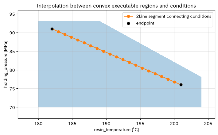

All points on the line segment can be executed: True

Reading the results

All orange line segments connecting two points within the blue region remain within the region. With this property, you can reduce the worry of sudden constraint violations caused by conditional interpolation. However, the ‘porous region’ where only the center of the temperature zone becomes unstable is non-convex. The definition of safety areas is verified not only by equipment specifications but also by the expertise of the quality assurance department.

No.052: What is a Convex Function?

Meaning in Practice

In a convex loss function, the loss when adopting the middle of extreme two conditions does not exceed the weighted average of losses at both ends. It makes it easier to assess the risks of changing conditions, and the direction of improvement is consistent.

Approach to Analysis and Modeling

If $f$ is convex if $f(\theta x+(1-\theta)y)\le\theta f(x)+(1-\theta)f(y)$ holds. In smooth quadratic functions, if all Hessian eigenvalues are non-negative, it is convex. Numerically check the curvature of this model and visualize the margins of Jensen’s inequality.

Check with Python

H = np.array([[5.2, -1.2], [-1.2, 4.2]])
eig = np.linalg.eigvalsh(H)
lhs = quality_loss(segment)
rhs = theta * quality_loss(A) + (1 - theta) * quality_loss(B)
display(pd.DataFrame({"Hessianeigenvalue": eig}).round(3))
plt.plot(theta, lhs, marker="o", label="Actual losses under intermediate conditions")
plt.plot(theta, rhs, "--", label="Weighted mean of endpoint loss (upper bound)")
plt.title("A convex function satisfiesJenseninequality")
plt.xlabel("endpointAMixing ratio θ"); plt.ylabel("Quality loss index")
plt.grid(True, alpha=0.3); plt.legend(); plt.tight_layout(); plt.show()
print(f"JensenMaximum number of inequalities violated: {np.max(lhs-rhs):.3e}")

	Hessianeigenvalue
0	3.4
1	6.0

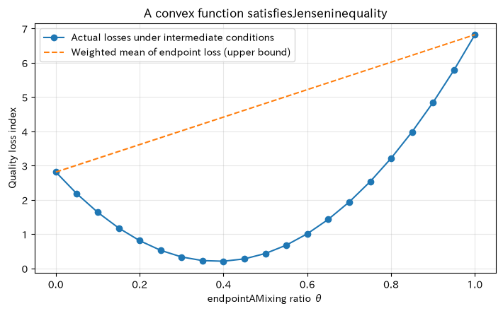
Maximum violation of Jensen's inequality: 0.000e+00

Reading the results

Hessian’s eigenvalues are both positive, and the actual loss is below the upper bound. Therefore, this model is narrowly convex and has only one valley bottom. In practice, even if the estimated response surface appears convex, it is not guaranteed to be outside the observation range. Leave uncertainties in the model ledger regarding the range of application and curvature.

No.053: Why Convex Optimization Is Important

Meaning in Practice

If the recommended conditions can be reached even if the person in charge or initial conditions change, the repeatability and auditability of the condition table improve. In convex problems, the locally optimal solution is also the global optimum, greatly reducing dependence on the search starting point.

Approach to Analysis and Modeling

Minimize the same convex objective function from different initial values and check the variation between the solution and the objective value. Since calculation tolerance remains, the physical unit is evaluated not as a perfect match but as a sufficiently small difference.

Check with Python

starts = np.array([[-1, -1], [-1, 1], [1.3, -0.8], [1.2, 1.1], [0, 0]])
rows = []
for s in starts:
    result = minimize(quality_loss, s, method="BFGS", options={"gtol": 1e-10})
    rows.append([*s, *result.x, result.fun, result.nit, result.success])
convex_runs = pd.DataFrame(rows, columns=["early stagex1", "early stagex2", "solutionx1", "solutionx2", "Final loss", "Repeated number", "Success"])
convex_runs["optimal_temperature_c"] = 190 + 10 * convex_runs["solutionx1"]
convex_runs["optimal_pressure_mpa"] = 80 + 10 * convex_runs["solutionx2"]
display(convex_runs.round(6))
print(f"Maximum difference between initial values: {np.ptp(convex_runs[['solutionx1','solutionx2']].to_numpy(), axis=0).max():.2e}")

	early stagex1	early stagex2	solutionx1	solutionx2	Final loss	Repeated number	Success	optimal_temperature_C	optimal_pressure_MPa
0	-1.0	-1.0	0.564706	0.447059	0.014118	5	False	195.647059	84.470588
1	-1.0	1.0	0.564706	0.447059	0.014118	6	True	195.647059	84.470588
2	1.3	-0.8	0.564706	0.447059	0.014118	4	False	195.647059	84.470588
3	1.2	1.1	0.564706	0.447059	0.014118	4	True	195.647059	84.470588
4	0.0	0.0	0.564706	0.447059	0.014118	6	True	195.647059	84.470588

Maximum difference between initial values: 1.45e-10

Reading the results

All starting points converge to almost the same conditions and losses. This is a reproducibility check that goes beyond the “solver marked as successful.” In production, the target value, constraint residual, stop reason, input data version, and solver version are also saved and recalculated.

No.054: Primary Conditions and Optimal Conditions

Meaning in Practice

We check that the recommended conditions are not just search results, but points that cannot be improved by minor changes to the conditions. In a condition change meeting, you can quantitatively respond to suggestions like “Wouldn’t it be better to raise the temperature a little?”

Approach to Analysis and Modeling

For differentiable convex functions, the necessary and sufficient condition for an unconstrained point $x^*$ to be optimal is $\nabla f(x^*)=0$. Also, the support hyperplane of the first order

$f(y)\ge f(x)+\nabla f(x)^\top(y-x)$

is valid in any $x,y$. Check the gradient norm and the primary lower bound.

Check with Python

def quality_grad(x):
    a, b = x
    return np.array([4 * (a - 0.6) + 1.2 * (a - b), 3 * (b - 0.4) - 1.2 * (a - b)])

x_star = minimize(quality_loss, [0, 0], jac=quality_grad, method="BFGS", tol=1e-12).x
x_base = np.array([-0.3, 0.8])
y_test = rng.uniform(-1, 1.3, size=(200, 2))
first_order_lower = quality_loss(x_base) + (y_test - x_base) @ quality_grad(x_base)
gap = quality_loss(y_test) - first_order_lower
display(pd.Series({
    "optimalx1": x_star[0], "optimalx2": x_star[1],
    "gradient norm": np.linalg.norm(quality_grad(x_star)),
    "Minimum margin for the first lower bound": gap.min(),
}).round(10))

Optimal x1 0.564706
Optimal x2 0.447059
Gradient Norm: 0.000000
Minimum margin of the first lower bound: 0.024987
dtype: float64

Reading the results

The gradient norm for the optimal point is almost zero, and at all tested points, the primary lower bound is less than the actual loss. If there is a constraint, the gradient may not reach zero, and in that case, the balance between the normal of the constraint and the target gradient, i.e., the KKT condition, is used to verify the calculation.

No.055: Duality and Lagrange Dual

Meaning in Practice

If the upper limit of the equipment load restricts optimal conditions, the value of slightly relaxing the limit can be expressed as an amount or loss index. This leads to prioritizing increased investment and bottleneck improvement.

Approach to Analysis and Modeling

To clarify the explanation, minimize the square distance to target condition $c=(0.9,0.7)$ and impose capability constraints $x_1+x_2\le b$.

$\min_x\ \frac12\lVert x-c\rVert^2,\qquad x_1+x_2-b\le0$

Minimizing Lagrangian $L(x,\lambda)=\frac12\lVert x-c\rVert^2+\lambda(x_1+x_2-b)$ with respect to $x$, the dual function is $g(\lambda)=-\lambda^2+\lambda(c_1+c_2-b)$. In any $\lambda\ge0$, $g(\lambda)$ is the lower bound of the principal problem optimal value.

Check with Python

c = np.array([0.9, 0.7]); capacity = 1.2
dual_lambda = np.linspace(0, 0.8, 161)
dual_value = -dual_lambda**2 + dual_lambda * (c.sum() - capacity)
lambda_star = (c.sum() - capacity) / 2
primal_x = c - lambda_star * np.ones(2)
primal_value = 0.5 * np.sum((primal_x - c)**2)
plt.plot(dual_lambda, dual_value, label="dual function g(λ)")
plt.axhline(primal_value, color="tab:red", linestyle="--", label="Optimal value for the main problem")
plt.scatter([lambda_star], [dual_value.max()], color="black", zorder=3)
plt.title("Lower bound of the optimal value by dual functions")
plt.xlabel("dual variable λ"); plt.ylabel("Target value／lower world")
plt.grid(True, alpha=0.3); plt.legend(); plt.tight_layout(); plt.show()
display(pd.Series({"optimalλ": lambda_star, "optimalx1": primal_x[0], "optimalx2": primal_x[1], "principal problem value": primal_value, "Double maximum": dual_value.max()}).round(4))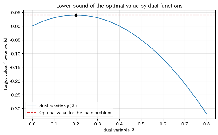

Optimal λ 0.20
Optimal x1 0.70
Optimal x2 0.50
Main problem value: 0.04
Double maximum value 0.04
dtype: float64

Reading the results

The dual function does not exceed the principal problem value for any non-negative λ and matches at optimal λ. λ is the rate of improvement in the target value when the capability limit is slightly relaxed. However, the scale depends on the unit of the objective function. If you use it for investment decisions, convert the quality loss index to yen and verify the sign and size even for finite differences.

No.056: Strong Duality

Meaning in Practice

If the best value of the main problem matches the lower bound of the dual problem, the quality of the solution can be numerically proven. Even for large-scale problems that cut off computation time, the dual gap serves as an indicator of “how much more room for improvement” remains.

Approach to Analysis and Modeling

In convex problems, if a Slater condition such as the Slater condition that there exists a point that strictly satisfies all inequality constraints holds, strong duality is obtained. In the previous question, $(0,0)$ satisfies $x_1+x_2<1.2$, so this condition is met. Change the ability cap and compare the main value, dual value, and sensitivity.

Check with Python

records = []
for b in [0.9, 1.0, 1.1, 1.2, 1.3, 1.4, 1.6, 1.8]:
    lam = max(0.0, (c.sum() - b) / 2)
    x = c - lam * np.ones(2)
    pv = 0.5 * np.sum((x - c)**2)
    dv = -lam**2 + lam * (c.sum() - b)
    records.append([b, *x, lam, pv, dv, pv-dv])
duality_df = pd.DataFrame(records, columns=["Ability Ceilingb", "x1", "x2", "λ", "principal problem value", "dual value", "Dual gap"])
display(duality_df.round(8))
plt.plot(duality_df["Ability Ceilingb"], duality_df["principal problem value"], "o-", label="Minimal loss")
plt.plot(duality_df["Ability Ceilingb"], duality_df["λ"], "s--", label="The Marginal Value of Constraint Relaxation λ")
plt.title("The relationship between facility capacity and losses and dual variables")
plt.xlabel("Ability Ceiling b"); plt.ylabel("Target value／dual variable")
plt.grid(True, alpha=0.3); plt.legend(); plt.tight_layout(); plt.show()

	Ability Ceilingb	x1	x2	λ	principal problem value	dual value	Dual gap
0	0.9	0.55	0.35	0.35	0.1225	0.1225	-0.0
1	1.0	0.60	0.40	0.30	0.0900	0.0900	0.0
2	1.1	0.65	0.45	0.25	0.0625	0.0625	0.0
3	1.2	0.70	0.50	0.20	0.0400	0.0400	0.0
4	1.3	0.75	0.55	0.15	0.0225	0.0225	0.0
5	1.4	0.80	0.60	0.10	0.0100	0.0100	0.0
6	1.6	0.90	0.70	0.00	0.0000	0.0000	0.0
7	1.8	0.90	0.70	0.00	0.0000	-0.0000	0.0

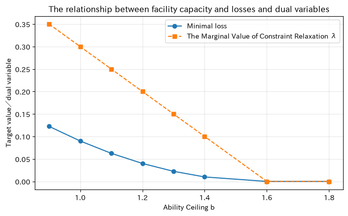
Reading the results

At all skill levels, the dual gap falls within the range of rounded error. The stricter the ability, the larger the λ, and the higher the marginal value of augmentation. If the upper limit exceeds the total target condition of 1.6, the constraint becomes inactive, and λ is zero. In practice, if the amplification is large at once, not only the local sensitivity λ but also the upper limit is adjusted and re-optimized after the increase.

No.057: Constrained Convex Optimization

Meaning in Practice

If the ideal conditions focused solely on quality are outside the equipment range, it cannot be implemented. Implementable conditions must be obtained that simultaneously satisfy the upper and lower limits of temperature and pressure, total load, and changes from standard conditions.

Approach to Analysis and Modeling

Combine linear inequality constraints with the convex objective function. We solve using SciPy’s SLSQP, but the results are checked not only by success flags but also by the margin for all constraints and comparison of target values with nearby candidates. Constraints are implemented in the form of $g(x)\ge0$.

Check with Python

constraints = [
    {"type": "ineq", "fun": lambda x: x[0] + 1.0},
    {"type": "ineq", "fun": lambda x: 1.4 - x[0]},
    {"type": "ineq", "fun": lambda x: x[1] + 1.0},
    {"type": "ineq", "fun": lambda x: 1.3 - x[1]},
    {"type": "ineq", "fun": lambda x: 0.75 - x[0] - x[1]},
]
r57 = minimize(quality_loss, [0, 0], jac=quality_grad, method="SLSQP", constraints=constraints,
               options={"ftol": 1e-12, "maxiter": 500})
margins = np.array([con["fun"](r57.x) for con in constraints])
display(pd.Series({
    "solver_success": r57.success, "optimal_temperature_c": 190 + 10*r57.x[0],
    "optimal_pressure_mpa": 80 + 10*r57.x[1], "quality_loss": r57.fun,
    "minimum constraint margin": margins.min(), "Repeated number": r57.nit,
}))

Z = quality_loss(np.stack([G1, G2], axis=-1))
plt.contour(190+10*G1, 80+10*G2, Z, levels=12, cmap="viridis")
mask57 = (G1 >= -1) & (G1 <= 1.4) & (G2 >= -1) & (G2 <= 1.3) & (G1 + G2 <= 0.75)
plt.contourf(190+10*G1, 80+10*G2, mask57.astype(int), levels=[0.5, 1.5], alpha=0.18, colors=["tab:blue"])
plt.scatter(190+10*r57.x[0], 80+10*r57.x[1], marker="*", s=180, color="tab:red", label="Constrained optimal solution")
plt.title("Minimizing quality loss within the executable area")
plt.xlabel("resin_temperature [°C]"); plt.ylabel("holding_pressure [MPa]")
plt.grid(True, alpha=0.3); plt.legend(); plt.tight_layout(); plt.show()

solver_success          True
Optimal temperature _C: 194.449153
Optimal pressure _MPa 83.050847
Quality loss 0.073347
Minimum constraint margin: 0.0
Number of Repetitions: 5
dtype: object

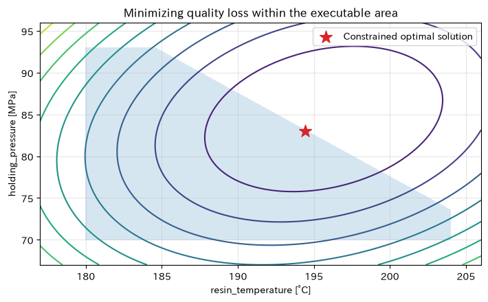
Reading the results

The optimal solution lies at the boundary of total load, and equipment capacity limits quality improvement. Since the minimum constraint margin is not negative, it is numerically feasible. However, considering control errors, you should not set boundary values as they are. In actual operation, safety margins are added according to temperature and pressure variations and further optimized under those conditions.

No.058: Regularization and Convex Optimization

Meaning in Practice

Proposals that drastically change conditions each time worsen setup load and site acceptance even if the quality is good. Regularization adjusts performance, “few changes,” and “simplicity of operation” using the same objective function.

Approach to Analysis and Modeling

Add L2 penalties to changes from the previous setting $x_{prev}=(-0.2,0.1)$.

$\min_x\ f(x)+\alpha\lVert x-x_{prev}\rVert_2^2$

The larger the $\alpha$, the more priority is given to maintaining the status quo. Since both are convex functions, the sum is also convex as well. Compare the trade-offs between quality loss and change volume across multiple $\alpha$.

Check with Python

x_prev = np.array([-0.2, 0.1])
reg_rows = []
for alpha in [0, 0.1, 0.3, 1, 3, 10]:
    objective = lambda x, a=alpha: quality_loss(x) + a*np.sum((x-x_prev)**2)
    r = minimize(objective, x_prev, method="BFGS")
    reg_rows.append([alpha, *r.x, quality_loss(r.x), np.linalg.norm(r.x-x_prev), r.fun])
reg_df = pd.DataFrame(reg_rows, columns=["Regularization strengthα", "x1", "x2", "quality_loss", "Amount of setting changes", "Objective value including regularization"])
display(reg_df.round(4))
plt.plot(reg_df["Amount of setting changes"], reg_df["quality_loss"], "o-")
for _, row in reg_df.iterrows():
    plt.annotate(f"α={row['Regularization strengthα']:g}", (row["Amount of setting changes"], row["quality_loss"]), xytext=(4, 4), textcoords="offset points")
plt.title("The trade-off between quality improvement and the amount of settings changed")
plt.xlabel("Number of changes since last setting"); plt.ylabel("Quality loss index")
plt.grid(True, alpha=0.3); plt.tight_layout(); plt.show()

	Regularization strengthα	x1	x2	quality_loss	Amount of setting changes	Objective value including regularization
0	0.0	0.5647	0.4471	0.0141	0.8398	0.0141
1	0.1	0.5308	0.4220	0.0174	0.7986	0.0812
2	0.3	0.4718	0.3805	0.0384	0.7280	0.1974
3	1.0	0.3259	0.2889	0.1696	0.5588	0.4819
4	3.0	0.1277	0.1915	0.5139	0.3402	0.8611
5	10.0	-0.0573	0.1294	0.9949	0.1457	1.2071

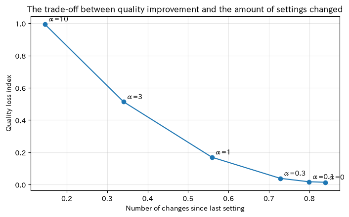
Reading the results

Strengthening regularization reduces the amount of setting changes but increases quality loss. α are not management decisions that are automatically determined by mathematics. If possible, the downtime required for changing conditions, verification costs, and work risks will be converted into yen and agreed upon as an operating policy. A design that separates α between regular and emergency revisions is also effective.

No.059: Lasso and Convex Optimization

Meaning in Practice

When quality is explained from multiple sensors, unnecessary signals enter the model, increasing maintenance costs and false alarms. Lasso reduces prediction errors while reducing some coefficients to zero, creating candidates to narrow down the monitoring targets.

Approach to Analysis and Modeling

Lasso is

$\min_{\beta_0,\beta}\ \frac{1}{2n}\lVert y-\beta_0-X\beta\rVert_2^2+\alpha\lVert\beta\rVert_1$

Solve it. Both the squared error and the L1 norm are convex values. To avoid unfairness due to unit differences, explanatory variables are standardized. Here, we generate fictitious data limited to four variables that truly affect the process: temperature, pressure, cooling time, and material moisture.

Check with Python

n_lasso, p = 160, 12
sensor_names = ["resin_temperature", "holding_pressure", "Cooldown time", "Material moisture", "Mold temperature", "injection velocity", "Back pressure", "outside temperature", "oil temperature", "vibration", "standby time", "lot number"]
X_sensor = rng.normal(size=(n_lasso, p))
true_beta = np.array([2.4, -1.8, 1.2, -0.9] + [0.0]*(p-4))
y_quality = 10 + X_sensor @ true_beta + rng.normal(0, 0.9, n_lasso)

lasso_rows = []
coef_paths = []
alphas = np.logspace(-2.2, 0.2, 20)
for alpha in alphas:
    model = make_pipeline(StandardScaler(), Lasso(alpha=alpha, max_iter=20000))
    model.fit(X_sensor, y_quality)
    coef = model[-1].coef_
    pred = model.predict(X_sensor)
    lasso_rows.append([alpha, np.count_nonzero(np.abs(coef) > 1e-8), np.sqrt(np.mean((y_quality-pred)**2))])
    coef_paths.append(coef)
lasso_df = pd.DataFrame(lasso_rows, columns=["α", "Nonzero coefficient number", "LearningRMSE"])
selected_idx = np.argmin(np.abs(alphas-0.18))
coef_table = pd.DataFrame({"Sensors": sensor_names, "Lassocoefficient": coef_paths[selected_idx], "True coefficient (at generation)": true_beta})
display(lasso_df.iloc[[0, 5, 10, 15, 19]].round(3))
display(coef_table.reindex(coef_table["Lassocoefficient"].abs().sort_values(ascending=False).index).round(3))

coef_paths = np.asarray(coef_paths)
for j, name in enumerate(sensor_names):
    plt.plot(alphas, coef_paths[:, j], label=name)
plt.xscale("log")
plt.title("LassoRegularization path")
plt.xlabel("Regularization strength α(Logarithmic line)"); plt.ylabel("Standardized regression coefficient")
plt.grid(True, alpha=0.3); plt.legend(bbox_to_anchor=(1.02, 1), loc="upper left", fontsize=8); plt.tight_layout(); plt.show()

	α	Nonzero coefficient number	LearningRMSE
0	0.006	12	0.893
5	0.027	8	0.898
10	0.116	4	0.940
15	0.495	4	1.452
19	1.585	1	2.778

	Sensors	Lassocoefficient	True coefficient (at generation)
0	resin_temperature	2.074	2.4
1	holding_pressure	-1.513	-1.8
2	Cooldown time	1.043	1.2
3	Material moisture	-0.766	-0.9
4	Mold temperature	-0.000	0.0
5	injection velocity	0.000	0.0
6	Back pressure	0.000	0.0
7	outside temperature	0.000	0.0
8	oil temperature	-0.000	0.0
9	vibration	-0.000	0.0
10	standby time	0.000	0.0
11	lot number	0.000	0.0

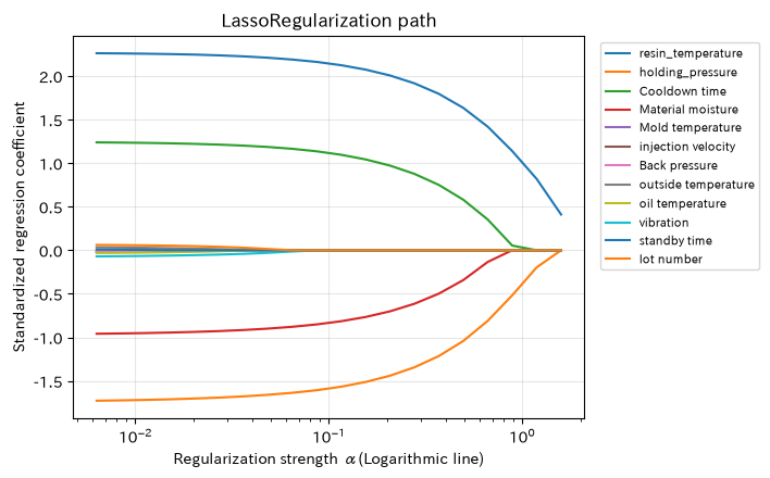
Reading the results

The stronger the α, the fewer nonzero coefficients decrease, while the four main variables remain relatively large. However, Lasso’s choice is not proof of causality. In strongly correlated sensor groups, representatives are replaced, and RMSE based solely on training data is optimistic. Selection is based on chronological verification, process knowledge, essential safety monitoring items, and alternatives in case of sensor failure.

No.060: Limits of Convex Optimization

Meaning in Practice

While convex models are easy to solve and explain, if a process includes multiple stable operating zones, whether or not there is a setup, an integer number of cars, or start/stop, it cannot fully represent reality. If you match the ‘solvable model’ to the actual site, it may look beautiful but may not be feasible.

Approach to Analysis and Modeling

Non-convex functions have multiple local solutions, and even if the first condition is met, it is not necessarily global optimal. For example, loss of a single variable

$h(z)=(z^2-1)^2+0.18z$

Let’s think about it. The second-order derivative $h''(z)=12z^2-4$ is negative near the origin and therefore nonconvex. Local optimization is performed from different initial values and compared to the best values of the global grid.

Check with Python

def nonconvex_loss(z):
    z = np.asarray(z)
    return (z**2 - 1)**2 + 0.18*z

z_grid = np.linspace(-1.8, 1.8, 1200)
nc_rows = []
for start in [-1.6, -0.5, 0.2, 0.8, 1.6]:
    r = minimize(lambda q: float(nonconvex_loss(q[0])), [start], method="BFGS")
    nc_rows.append([start, r.x[0], r.fun, r.success])
nc_df = pd.DataFrame(nc_rows, columns=["initial value", "arrival point", "local objective value", "Success"])
global_i = np.argmin(nonconvex_loss(z_grid))
display(nc_df.round(5))
print(f"Best candidates for the global grid confirmed: z={z_grid[global_i]:.4f}, loss={nonconvex_loss(z_grid[global_i]):.4f}")
plt.plot(z_grid, nonconvex_loss(z_grid), label="Non-convex process losses")
plt.scatter(nc_df["arrival point"], nc_df["local objective value"], color="tab:red", zorder=3, label="Points from each initial value")
plt.title("In non-convex problems, the initial value changes the reached solution")
plt.xlabel("Standardized process conditions z"); plt.ylabel("loss index")
plt.grid(True, alpha=0.3); plt.legend(); plt.tight_layout(); plt.show()

	initial value	arrival point	local objective value	Success
0	-1.6	-1.02178	-0.18198	True
1	-0.5	-1.02178	-0.18198	True
2	0.2	0.97669	0.17793	True
3	0.8	0.97669	0.17793	True
4	1.6	0.97669	0.17793	True

Best global candidates confirmed on the grid: z = -1.0224, loss = -0.1820

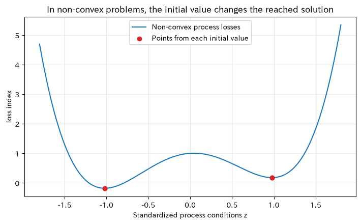
Reading the results

Even if solvers “succeed” at each starting point, they will reach different valleys on the left and right, with different target values. If nonconvexity is suspected, consider multi-point initialization, global search, mixed integer optimization, simulation, and expert candidate area segmentation. When using convex approximation, the feasibility and optimality gap against the original constraint are evaluated separately.

Practical Implications Seen Through Target Exercise

1. First, check the convexity: Checking the executable domain and the structure of the objective function changes not only the solution method but also the explainability.
2. Prioritize validation over optimal values: Gradients, constraint margins, dual gaps, and results from different initial values.
3. Connecting dual variables to investment decisions: Convert the mitigated value of activation constraints into yen and compare candidates for capacity enhancement.
4. Designing Regularization as an Operational Cost: Explicitly incorporate settings for changes, sensor maintenance, and model complexity.
5. Don’t hide the reality that isn’t convex: If there are planning, integer determination, multiple driving zones, or discontinuous quality judgments, you need a different model or solution.

What is necessary for practical implementation

• Agreement on objective functions: Defects, reprocessing, power consumption, downtime, and delivery delays are converted into common units and approved across departments.
• Ledger of constraints: Manage the basis, responsible person, and update date regarding equipment limits, quality standards, safety margins, and possible change ranges.
• Checking Data Quality: Audit calibration history, missing measurements, time synchronization, lot differences, and the scope of operation for condition changes.
• Offline Verification: Testing reproduction with historical data, sensitivity analysis, extrapolation detection, and fail-safe during abnormal inputs
• On-site Verification Tests: Gradually test recommended conditions and evaluate standard margins, including control variation.
• Operational Monitoring: Record objective values, constraint margins, input distribution, forecast errors, and reasons for re-optimization, and reflect them with approval.

Conclusion

Convex optimization is not simply a method that solves quickly. It is a decision-making framework that can consistently explain safe condition areas, loss patterns, optimality conditions, and the value of constraints. In this article, we reviewed everything from convex sets and convex functions to strong duality, constrained optimization, Lasso, and key points for non-convex problems, all through the flow of molding condition design. In practice, it is important to separate and verify the convexity of the model from its real-world validity, and to translate the optimal solution into conditions that can be safely implemented.

Consultations for Corporations

At Suri Kobo, we support everything from problem organization to PoC and production operation design, covering the integration of manufacturing condition optimization, production planning, equipment capability evaluation, and quality forecasting and optimization. You can consult with us starting from the stages of “how to define objective functions” and “how to model constraints and on-site rules.”

📩 Contact Us: surikobo.co.jp/contact Please feel free to consult us first.