Anticipating Demand Fluctuations and Equipment Deterioration: Dynamic Planning and Sequential Decision-Making 10 Exercises

Set in a fictional precision parts factory, it handles production, inventory, and equipment maintenance with The impact of this week’s decision on next week and beyond incorporated. The target is No.061〜No.070(Dynamic Planning and Sequential Decision-Making).

[!NOTE] This material is a notebook previously used by Surikoubo (or personally by the representative, Kazuyama), and has been reconstructed, edited, and published with the company’s permission.
All data listed is fictional and has no relation whatsoever to real companies, factories, or figures.

Introduction: Practical Challenges in Manufacturing Covered in This Article

On the manufacturing floor, increasing production, holding inventory, preventive maintenance, and equipment upgrades cannot be evaluated in a single period. This article discusses dynamic programming, which selects current actions including future costs; DP) with small, traceable examples.

Common situations on site

• Overproduction to avoid stockouts increases inventory costs and the risk of retention
• If maintenance is postponed, it can operate this week, but the probability of failure and downtime losses will increase.
• Extending the lifespan of aging equipment improves short-term financial balances while driving up future maintenance costs.
• Because conditions and demands change, fixed rules are not always the best

Why is this issue so difficult to judge?

This is because the effects of actions span time and carry uncertainty. Sequential decision-making compares “current costs” and “future value after action” on the same scale. However, as states, actions, and periods increase, combinations increase rapidly, so model granularity is also an important design decision.

Overview of Exercise covered this time

No.	Theme	Judgment in the manufacturing industry
061	What is dynamic programming?	Determining the production volume over multiple periods
062	Bellman Equation	Separating current expenses from future value
063	Shortest Route and Dynamic Programming	Evaluating process routes from behind
064	The Knapsack Problem and Dynamic Programming	Select improvement projects within your budget
065	Inventory Management and Dynamic Planning	Determining order quantities under demand fluctuations
066	Equipment Upgrade Issues	Compare repair, continuation, and renewal
067	Markov Decision Process	Handling Probabilistic Transitions of Equipment States
068	value repetition method	Seeking solutions with low long-term costs
069	Strategy Iterative Method	Separating measure evaluation from improvement
070	Relationship with Reinforcement Learning	Learning Unknown Transitions from Driving Data

Preparing the Python environment

No external data is used. Fix the random number seed so you can reproduce the same result. For clarity, the amount is in thousand yen units.

import platform
import numpy as np
import pandas as pd
import matplotlib
import matplotlib.pyplot as plt
from IPython.display import display

rng = np.random.default_rng(42)
plt.rcParams["figure.figsize"] = (7.2, 4.5)
plt.rcParams["axes.unicode_minus"] = False

pd.DataFrame({
    "package": ["Python", "NumPy", "pandas", "Matplotlib"],
    "version": [platform.python_version(), np.__version__, pd.__version__, matplotlib.__version__],
})

	package	version
0	Python	3.13.1
1	NumPy	2.5.1
2	pandas	3.0.3
3	Matplotlib	3.11.0

Creation of Fictional Data

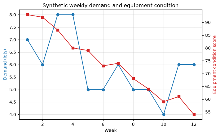
Assume a 12-week precision parts factory. Demand fluctuates gently and randomly, while equipment experiences weekly deterioration. This observation table is for contextual understanding, and for each subsequent exercise, small models are also used to separate decision-making issues.

weeks = np.arange(1, 13)
demand = np.maximum(2, np.rint(6 + 1.5*np.sin(weeks/2) + rng.normal(0, 1.0, len(weeks)))).astype(int)
condition = np.maximum(45, np.rint(96 - 3.5*weeks + rng.normal(0, 2.5, len(weeks)))).astype(int)
factory = pd.DataFrame({"week": weeks, "demand_lots": demand, "equipment_condition": condition})
display(factory)

fig, ax1 = plt.subplots()
ax1.plot(weeks, demand, marker="o", label="Demand", color="tab:blue")
ax1.set_xlabel("Week"); ax1.set_ylabel("Demand (lots)", color="tab:blue")
ax2 = ax1.twinx(); ax2.plot(weeks, condition, marker="s", label="Condition", color="tab:red")
ax2.set_ylabel("Equipment condition score", color="tab:red")
ax1.set_title("Synthetic weekly demand and equipment condition")
ax1.grid(True, alpha=.3); fig.tight_layout(); plt.show()

	week	demand_lots	equipment_condition
0	1	7	93
1	2	6	92
2	3	8	87
3	4	8	80
4	5	5	79
5	6	5	73
6	7	6	74
7	8	5	68
8	9	5	64
9	10	4	59
10	11	6	61
11	12	6	54

No.061: What is Dynamic Programming?

Meaning in Practice

Dynamic planning divides multi-period problems into “states” and “actions,” reusing the same subproblems. Here, starting inventory is considered the condition, production volume is the action, and production costs are minimized over three weeks.

Approach to Analysis and Modeling

If demand is $d_t$, beginning inventory is $s_t$, and production volume is $a_t$, the status is updated at $s_{t+1}=s_t+a_t-d_t$. The value function $V_t(s)$ is the minimum cumulative cost that can be achieved after point $t$.

$V_t(s)=\min_a\{c_t(a)+h(s+a-d_t)+V_{t+1}(s+a-d_t)\}$

Check with Python

dp_demand = [4, 7, 5]
capacity, max_inventory = 8, 8
unit_cost, holding_cost = [5, 8, 6], 1.2
V = {3: {s: 0.0 for s in range(max_inventory + 1)}}
policy = {}
for t in range(2, -1, -1):
    V[t], policy[t] = {}, {}
    for s in range(max_inventory + 1):
        choices = []
        for a in range(capacity + 1):
            nxt = s + a - dp_demand[t]
            if 0 <= nxt <= max_inventory:
                choices.append((unit_cost[t]*a + holding_cost*nxt + V[t+1][nxt], a))
        if choices:
            V[t][s], policy[t][s] = min(choices)

s, plan = 0, []
for t in range(3):
    a = policy[t][s]; nxt = s + a - dp_demand[t]
    plan.append([t+1, s, dp_demand[t], a, nxt, unit_cost[t]*a + holding_cost*nxt])
    s = nxt
display(pd.DataFrame(plan, columns=["week","opening_inventory","demand","production","closing_inventory","current_cost_kJPY"]))
print(f"Minimum 3-week cost: {V[0][0]:.1f} kJPY")

	week	opening_inventory	demand	production	closing_inventory	current_cost_kJPY
0	1	0	4	8	4	44.8
1	2	4	7	3	0	24.0
2	3	0	5	5	0	30.0

Minimum 3-week cost: 98.8 kJPY

Reading the results

Because the unit price in the second week is high, models are produced ahead of schedule in the first week to keep inventory. This is an effect that cannot be seen by deciding to set the lowest price only for each week. On the other hand, if storage capacity, yield, arrangement, and shortage tolerance are excluded, the plan becomes unfeasible, so it is necessary to check state transitions and constraints.

No.062: Bellman’s Equation

Meaning in Practice

The Bellman equation divides current actions into “costs that occur now” and “future costs in the next state.” This breakdown explains why you chose that production volume.

Approach to Analysis and Modeling

If you set the total evaluation value for candidate action $a$ as $Q_t(s,a)=c_t(s,a)+V_{t+1}(f(s,a))$, it is $V_t(s)=\min_a Q_t(s,a)$. The principle of optimality states that the remaining parts of the optimal plan are also optimal from the perspective of their reached state.

Check with Python

t, s = 0, 0
rows = []
for a in range(capacity + 1):
    nxt = s + a - dp_demand[t]
    if nxt in V[t+1]:
        immediate = unit_cost[t]*a + holding_cost*nxt
        rows.append([a, nxt, immediate, V[t+1][nxt], immediate + V[t+1][nxt]])
bellman = pd.DataFrame(rows, columns=["production","next_inventory","immediate_cost","future_cost","total_Q"])
display(bellman.round(1))
bellman.set_index("production")[["immediate_cost","future_cost"]].plot(kind="bar", stacked=True)
plt.title("Bellman decomposition at week 1"); plt.xlabel("Production (lots)"); plt.ylabel("Cost (kJPY)")
plt.grid(True, axis="y", alpha=.3); plt.tight_layout(); plt.show()

	production	next_inventory	immediate_cost	future_cost	total_Q
0	4	0	20.0	86.0	106.0
1	5	1	26.2	78.0	104.2
2	6	2	32.4	70.0	102.4
3	7	3	38.6	62.0	100.6
4	8	4	44.8	54.0	98.8

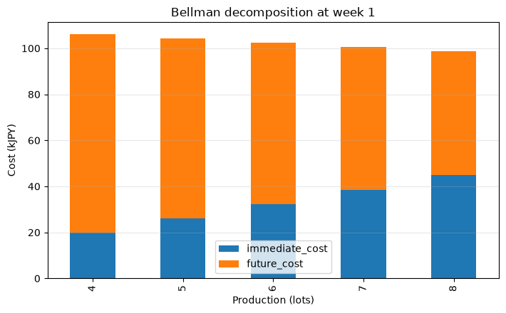
Reading the results

The more production volume increases, the higher current cost increases, but since you can avoid high-price weeks, future costs decrease. The minimum total action is adopted. During the site briefing, presenting this breakdown makes it easier to share “why we are making extra now.”

No.063: Shortest Path and Dynamic Programming

Meaning in Practice

Route selection for products passing through multiple processes can be represented as dynamic planning, with the current location as the state and the next chosen process as the action. Process time, outsourcing costs, and quality risks are converted into common costs.

Approach to Analysis and Modeling

With directed acyclic graphs, you can calculate $V(i)=\min_{j\in N(i)}\{c_{ij}+V(j)\}$ in reverse order from the endpoint. For general graphs without negative edges, choose solutions that fit the problem structure, such as the Dijkstra method.

Check with Python

edges = {
    "Material": [("Cut-A", 4.0), ("Cut-B", 5.0)],
    "Cut-A": [("Heat-1", 7.0), ("Heat-2", 5.0)],
    "Cut-B": [("Heat-1", 4.0), ("Heat-2", 6.0)],
    "Heat-1": [("Inspect", 3.0)], "Heat-2": [("Inspect", 4.0)],
    "Inspect": [("Ship", 2.0)], "Ship": []}
order = ["Ship","Inspect","Heat-2","Heat-1","Cut-B","Cut-A","Material"]
route_value, next_node = {"Ship": 0.0}, {}
for node in order[1:]:
    route_value[node], next_node[node] = min((cost + route_value[j], j) for j, cost in edges[node])
path, node = ["Material"], "Material"
while node != "Ship": node = next_node[node]; path.append(node)
display(pd.DataFrame({"node": list(route_value), "minimum_remaining_cost": list(route_value.values())}).sort_values("minimum_remaining_cost"))
print("Best route:", " -> ".join(path), f" / cost={route_value['Material']:.1f}")

	node	minimum_remaining_cost
0	Ship	0.0
1	Inspect	2.0
3	Heat-1	5.0
2	Heat-2	6.0
4	Cut-B	9.0
5	Cut-A	11.0
6	Material	14.0

Best route: Material -> Cut-B -> Heat-1 -> Inspect -> Ship  / cost=14.0

Reading the results

The minimum residual cost from each process to shipment can be determined, allowing you to restore the optimal route. When adding quality loss or lead time to the cost coefficient, the basis for the amount conversion and the prohibition or capability limit are separately managed.

No.064: The Knapsack Problem and Dynamic Programming

Meaning in Practice

When the improvement budget is limited, ranking projects based solely on effect amounts may waste budget combinations. The 0-1 knapsack problem determines the acceptance or rejection of each project simultaneously.

Approach to Analysis and Modeling

The investment amount for Project $i$ is $w_i$, annual effectiveness is $v_i$, budget is $B$, and $\max\sum_i v_i x_i$, $\sum_i w_i x_i\le B$, and $x_i\in\{0,1\}$ are set. DP preserves the value of “top $i$ cases, remaining budget $b$.”

Check with Python

projects = pd.DataFrame({
    "project": ["Vision inspection","Tool monitoring","Energy control","AGV routing","Predictive maintenance"],
    "investment": [6, 4, 3, 5, 7], "annual_benefit": [11, 7, 5, 9, 13]})
B, n = 12, len(projects)
table = np.zeros((n+1, B+1), dtype=int)
for i in range(1, n+1):
    w, v = projects.loc[i-1, ["investment","annual_benefit"]]
    for b in range(B+1):
        table[i,b] = table[i-1,b]
        if w <= b: table[i,b] = max(table[i,b], table[i-1,b-w] + v)
b, chosen = B, []
for i in range(n, 0, -1):
    if table[i,b] != table[i-1,b]: chosen.append(i-1); b -= projects.loc[i-1,"investment"]
display(projects.assign(selected=[i in chosen for i in range(n)]))
print(f"Investment={projects.loc[chosen,'investment'].sum()}, benefit={table[n,B]}")
plt.plot(range(B+1), table[n], marker="o"); plt.title("Best annual benefit by investment budget")
plt.xlabel("Budget"); plt.ylabel("Maximum annual benefit"); plt.grid(True, alpha=.3); plt.tight_layout(); plt.show()

	project	investment	annual_benefit	selected
0	Vision inspection	6	11	False
1	Tool monitoring	4	7	False
2	Energy control	3	5	False
3	AGV routing	5	9	True
4	Predictive maintenance	7	13	True

Investment=12, benefit=22

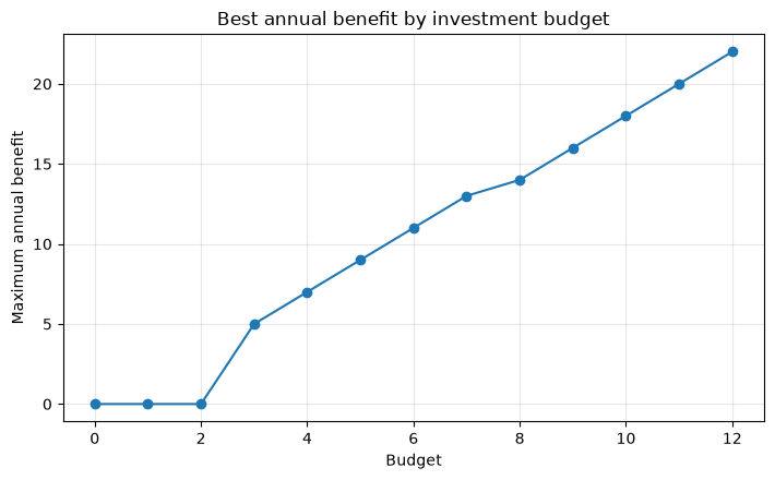
Reading the results

The adoption set is the most effective combination across the entire budget. If the effect amount is uncertain, depends between projects, personnel implementing personnel, or cannot be implemented simultaneously, these are extended to scenario analysis and integer planning.

No.065: Inventory Management and Dynamic Planning Method

Meaning in Practice

For parts whose demand is not yet certain, the order quantity is determined by considering not only inventory costs but also shortage costs. Shortage fees reflect express shipping, line stoppages, and delivery delays.

Approach to Analysis and Modeling

If demand $D_t$ is a random variable, then the Bellman equation containing the expected value

$V_t(s)=\min_a\left\{K\mathbf{1}_{a>0}+ca+\mathbb E[h(s+a-D_t)^++p(D_t-s-a)^++V_{t+1}((s+a-D_t)^+)]\right\}$

We use it. Here, unmet demand is treated as a shortage for the current period and will not be carried over to the next period.

Check with Python

dvals, probs = np.array([2,4,6,8]), np.array([.15,.35,.35,.15])
T, Smax, Amax = 3, 12, 10
fixed, purchase, hold, shortage = 6.0, 3.0, 1.0, 9.0
IV = {T: np.zeros(Smax+1)}; IP = {}
for t in range(T-1, -1, -1):
    IV[t], IP[t] = np.zeros(Smax+1), np.zeros(Smax+1, dtype=int)
    for s in range(Smax+1):
        qvals = []
        for a in range(Amax+1):
            if s+a > Smax: continue
            exp = fixed*(a>0) + purchase*a
            for d, pr in zip(dvals, probs):
                nxt=max(s+a-d,0); lost=max(d-s-a,0)
                exp += pr*(hold*nxt + shortage*lost + IV[t+1][nxt])
            qvals.append((exp,a))
        IV[t][s], IP[t][s] = min(qvals)
inventory_policy = pd.DataFrame({"opening_inventory":range(Smax+1),"order_week1":IP[0],"expected_cost_to_go":IV[0]})
display(inventory_policy.round(2))
plt.step(inventory_policy.opening_inventory, inventory_policy.order_week1, where="mid")
plt.title("Inventory-dependent ordering policy"); plt.xlabel("Opening inventory (lots)"); plt.ylabel("Order quantity (lots)")
plt.grid(True, alpha=.3); plt.tight_layout(); plt.show()

	opening_inventory	order_week1	expected_cost_to_go
0	0	8	73.07
1	1	7	70.07
2	2	6	67.07
3	3	5	64.07
4	4	0	60.80
5	5	0	55.30
6	6	0	49.80
7	7	0	46.58
8	8	0	43.07
9	9	0	40.66
10	10	0	37.33
11	11	0	35.03
12	12	0	31.33

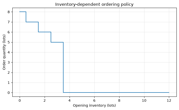
Reading the results

When inventory is low, orders are placed in bulk, and orders are not placed above a certain level. Because there are fixed order costs, it is not a simple replenishment every fiscal year. In practice, we also verify updates on demand distribution, order lead times, lot rounding, storage periods, and service levels.

No.066: Equipment Update Issue

Meaning in Practice

Equipment renewal involves comparing not only the purchase price but also maintenance costs due to aging, downtime losses, and residual value after renewal over multiple years.

Approach to Analysis and Modeling

The equipment age is the state: if it is “continuous,” the age increases by 1; if “renewed,” the age of the new equipment will be 1 in the next term. Compare at present value based on a discount rate of $r$, and place residual value at the endpoint.

Check with Python

horizon, max_age, discount = 5, 8, .95
replace_cost = 65.0
maintenance = np.array([5 + 2*a + .8*a*a for a in range(max_age+2)])
EV = {horizon: {a: -max(3, 18-2*a) for a in range(max_age+1)}}
EP = {}
for t in range(horizon-1, -1, -1):
    EV[t], EP[t] = {}, {}
    for age in range(max_age+1):
        keep = maintenance[age] + discount*EV[t+1][min(age+1,max_age)]
        replace = replace_cost + maintenance[0] + discount*EV[t+1][1]
        EV[t][age], EP[t][age] = min((keep,"Keep"),(replace,"Replace"))
eq = pd.DataFrame({"equipment_age":range(max_age+1),"decision_now":[EP[0][a] for a in range(max_age+1)],"discounted_cost":[EV[0][a] for a in range(max_age+1)]})
display(eq.round(1))
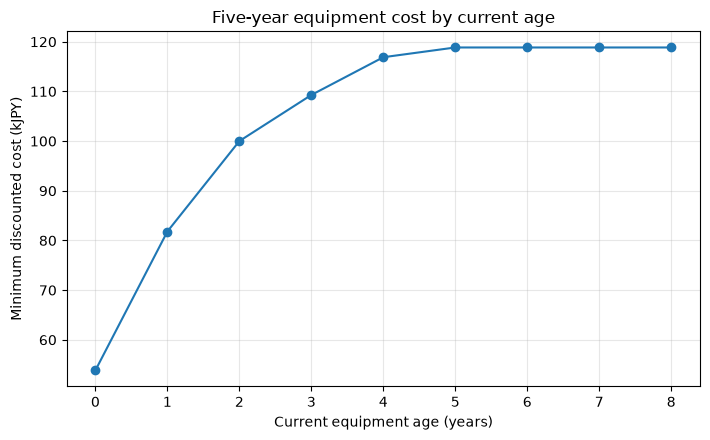
plt.plot(eq.equipment_age, eq.discounted_cost, marker="o"); plt.title("Five-year equipment cost by current age")
plt.xlabel("Current equipment age (years)"); plt.ylabel("Minimum discounted cost (kJPY)")
plt.grid(True, alpha=.3); plt.tight_layout(); plt.show()

	equipment_age	decision_now	discounted_cost
0	0	Keep	53.8
1	1	Keep	81.8
2	2	Keep	100.0
3	3	Keep	109.3
4	4	Keep	116.9
5	5	Replace	118.8
6	6	Replace	118.8
7	7	Replace	118.8
8	8	Replace	118.8

Reading the results

Young equipment continues and is replaced as it ages. Since thresholds vary depending on maintenance costs, renewal costs, discount rates, and residual value, a sensitivity table should be attached to the capital investment review rather than a single conclusion.

No.067: Markov Decision Process

Meaning in Practice

The Markov Decision Process (MDP) represents the condition of equipment as a state of health, deterioration, or failure, and the probability of the next state changes depending on operation, maintenance, and replacement.

Approach to Analysis and Modeling

MDPs consist of state $S$, action $A$, transition probability $P(s'|s,a)$, cost $c(s,a)$, and discount rate $\gamma$. Markov behavior assumes that the necessary historical information is summarized into the current state.

Check with Python

states = ["Healthy","Degraded","Failed"]
actions = ["Run","Maintain","Replace"]
P = np.array([
 [[.85,.14,.01],[.95,.05,0],[1,0,0]],
 [[.25,.55,.20],[.75,.23,.02],[1,0,0]],
 [[0,0,1],[.55,.40,.05],[1,0,0]]])
C = np.array([[2,8,25],[5,10,25],[45,35,25]], dtype=float)
rows=[]
for si,s in enumerate(states):
 for ai,a in enumerate(actions): rows.append([s,a,C[si,ai],*P[si,ai]])
mdp_table=pd.DataFrame(rows,columns=["state","action","cost","P_healthy","P_degraded","P_failed"])
display(mdp_table)
print("Maximum transition-row error:", np.abs(P.sum(axis=2)-1).max())

	state	action	cost	P_healthy	P_degraded	P_failed
0	Healthy	Run	2.0	0.85	0.14	0.01
1	Healthy	Maintain	8.0	0.95	0.05	0.00
2	Healthy	Replace	25.0	1.00	0.00	0.00
3	Degraded	Run	5.0	0.25	0.55	0.20
4	Degraded	Maintain	10.0	0.75	0.23	0.02
5	Degraded	Replace	25.0	1.00	0.00	0.00
6	Failed	Run	45.0	0.00	0.00	1.00
7	Failed	Maintain	35.0	0.55	0.40	0.05
8	Failed	Replace	25.0	1.00	0.00	0.00

Maximum transition-row error: 0.0

Reading the results

Even with the same ‘operation,’ the probability of failure is high when deteriorated, and maintenance pays for improvements in transitions. If the state definition is too coarse, Markov disrupts the principle. We verify whether information necessary for future forecasting, such as vibration, cumulative operation, and near-term maintenance, is included in the condition.

No.068: Value Repetition Method

Meaning in Practice

The value iteration method repeatedly updates the long-term costs of each state and seeks actions with minimal cost. This forms the basis for establishing standard response rules for each equipment condition.

Approach to Analysis and Modeling

For the indefinite period problem with a discount rate $\gamma$,

$V_{k+1}(s)=\min_a\{c(s,a)+\gamma\sum_{s'}P(s'|s,a)V_k(s')\}$

Repeat until convergence. Residuals are an indicator of numerical convergence and do not guarantee model validity.

Check with Python

gamma = .95
value = np.zeros(len(states)); residuals=[]
for k in range(1000):
    Q = C + gamma*np.einsum("sak,k->sa", P, value)
    new_value = Q.min(axis=1)
    residuals.append(np.max(np.abs(new_value-value)))
    value = new_value
    if residuals[-1] < 1e-10: break
vi_policy = Q.argmin(axis=1)
display(pd.DataFrame({"state":states,"long_run_cost":value,"recommended_action":[actions[i] for i in vi_policy]}).round(2))
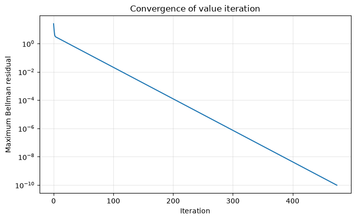
plt.semilogy(residuals); plt.title("Convergence of value iteration"); plt.xlabel("Iteration"); plt.ylabel("Maximum Bellman residual")
plt.grid(True, alpha=.3); plt.tight_layout(); plt.show()
print("Iterations:", len(residuals))

	state	long_run_cost	recommended_action
0	Healthy	67.97	Run
1	Degraded	76.94	Maintain
2	Failed	89.57	Replace

Iterations: 475

Reading the results

You can get condition-dependent strategies: operation when healthy, maintenance when deteriorating, and replacement when broken. The closer the discount rate is to 1, the more distant the future is emphasized, and the longer it converges. We also check the stability of measures that change costs and transition probabilities.

No.069: Strategy Iterative Method

Meaning in Practice

The Iterative Approach evaluates the long-term costs of current standard rules and only changes actions where improvement is possible. The comparison with current measures is clear.

Approach to Analysis and Modeling

Fix $\pi$ to solve $(I-\gamma P_\pi)V_\pi=c_\pi$ and use its value to improve behavior in each state. If the strategy no longer changes, it will end.

Check with Python

pi = np.array([0,0,1])  # Healthy=Run, Degraded=Run, Failed=Maintain
history=[]
for it in range(20):
    Ppi=P[np.arange(3),pi]; cpi=C[np.arange(3),pi]
    vpi=np.linalg.solve(np.eye(3)-gamma*Ppi,cpi)
    qpi=C+gamma*np.einsum("sak,k->sa",P,vpi)
    improved=qpi.argmin(axis=1)
    history.append([it,*[actions[x] for x in pi],*vpi])
    if np.array_equal(improved,pi): break
    pi=improved
display(pd.DataFrame(history,columns=["iteration","Healthy_action","Degraded_action","Failed_action","V_healthy","V_degraded","V_failed"]).round(2))
print("Stable policy:", dict(zip(states,[actions[x] for x in pi])))

	iteration	Healthy_action	Degraded_action	Failed_action	V_healthy	V_degraded	V_failed
0	0	Run	Run	Maintain	90.65	106.94	129.14
1	1	Run	Maintain	Replace	67.97	76.94	89.57

Stable policy: {'Healthy': 'Run', 'Degraded': 'Maintain', 'Failed': 'Replace'}

Reading the results

From the initial current rules, through evaluation and improvement, we reach the same approach as value iteration. If the number of states is large, the problem of solving linear equations increases, so iterative evaluation and approximation methods are considered.

No.070: Relationship with Reinforcement Learning

Meaning in Practice

DP and MDP assume that transition probabilities and cost models are known. Reinforcement learning estimates value based on the “state, behavior, cost, and next state” obtained through trials. Here, we will learn the same maintenance problems using Q-learning.

Approach to Analysis and Modeling

The cost-minimized version of Q-learning is based on observation samples.

$Q(s,a)\leftarrow Q(s,a)+\alpha\{c+\gamma\min_{a'}Q(s',a')-Q(s,a)\}$

I will update you. No model is required, but safe and sufficient exploration is required. This does not mean unlimited exploration on the actual device.

Check with Python

qrng=np.random.default_rng(42); Qlearn=np.zeros((3,3)); visits=np.zeros((3,3),int)
episodes, steps = 12000, 25
agreement=[]
for ep in range(episodes):
    s=int(qrng.integers(0,3)); eps=max(.03, .8*(1-ep/episodes))
    for _ in range(steps):
        a=int(qrng.integers(0,3)) if qrng.random()<eps else int(np.argmin(Qlearn[s]))
        sn=int(qrng.choice(3,p=P[s,a])); cost=C[s,a]; visits[s,a]+=1
        alpha=max(.02, .5/(visits[s,a]**.55))
        Qlearn[s,a]+=alpha*(cost+gamma*Qlearn[sn].min()-Qlearn[s,a]); s=sn
    agreement.append(np.mean(Qlearn.argmin(axis=1)==vi_policy))
learned=Qlearn.argmin(axis=1)
display(pd.DataFrame({"state":states,"MDP_action":[actions[i] for i in vi_policy],"learned_action":[actions[i] for i in learned],"minimum_visits":visits.min(axis=1)}))
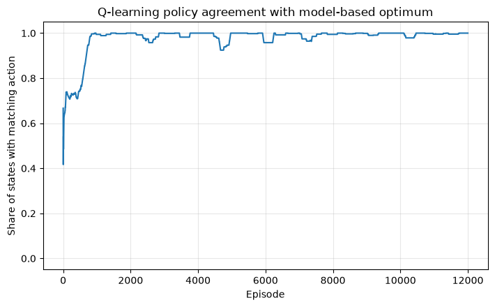
plt.plot(pd.Series(agreement).rolling(300,min_periods=1).mean()); plt.title("Q-learning policy agreement with model-based optimum")
plt.xlabel("Episode"); plt.ylabel("Share of states with matching action"); plt.ylim(-.05,1.05)
plt.grid(True, alpha=.3); plt.tight_layout(); plt.show()

	state	MDP_action	learned_action	minimum_visits
0	Healthy	Run	Run	33523
1	Degraded	Maintain	Maintain	5006
2	Failed	Replace	Replace	1222

Reading the results

With sufficient simulation experience, the learning strategies align with those obtained from known models. However, in practice, challenges include insufficient learning for low-frequency failures, distribution changes due to equipment changes, safety constraints, and search costs. First, it is practical to introduce stages that use simulators, historical logs, and offline evaluations to retain human approval.

Practical Implications Seen Through Target Exercise

• Sequential decision-making evaluates not only current fiscal year KPIs but also the future value of the following state
• Conditions are narrowed down to providing sufficient information for future forecasts, preventing an explosion in the number of states.
• Prepare explanatory materials not only for optimal measures but also for immediate costs, future costs, and differences from alternative actions
• Transition probabilities, demand distribution, and cost factors are regularly re-estimated to monitor changes in strategy
• Rather than a simple binary of DP/MDP if the model is known, or learning if unknown, it combines known information with data.
• Reinforcement learning exploration is conducted under simulators or safety constraints, without directly connecting to actual machines

What is necessary for practical implementation

Points of Contention	confirmation item	Main Deliverables
Decision-making	Who chooses, when, and what	Business Flow & Approval Responsibilities
Condition	How to represent inventory, deterioration, work-in-progress, and delivery dates	State Definition & Data Dictionary
Actions and Constraints	Capacity, safety, lots, and preservation windows	List of Constraints and Rationale
Fees	Out-of-stock, discontinuous, quality, residual value	Cost Conversion Table & Sensitivity Analysis
probability	Demand and Fault Transition Estimation Accuracy	Estimation Procedure & Verification Results
Utilization	Recalculation, exceptions, model degradation	SOP and Monitoring Dashboard

Initially, limit the number of states and actions, then use the current rules as a baseline for backtesting with past data. Starting with decision support where people confirm reasons for recommendations and alternatives, it simultaneously monitors downtime losses, service levels, and workload.

Conclusion

Multi-period production, process routes, improvement projects, inventory, and equipment renewals are represented as DP, and probabilistic equipment maintenance is expanded into MDP, value iteration, policy iteration, and Q-learning. What matters is not the advanced solution itself, but the clarity of the carryover effects as state transitions, making them decision-making rules that can be verified by the field.

Consultations for Corporations

At Surikoubo, we support sequential decision-making in production, inventory, and equipment maintenance, including problem organization, data design, simulation, optimization PoC, and operational design.

📩 Contact Us: surikobo.co.jp/contact
Please feel free to consult us first.