Determining machining conditions with data: 10-step exercises that balance quality, power, and constraints through nonlinear optimization

Using a fictional resin molding process as the subject, we handle setting conditions that comply with equipment constraints while minimizing quality loss and electricity costs. The target is No.041〜No.050(Nonlinear optimization).

[!NOTE] This material is a notebook previously used by Surikoubo (or personally by the representative, Kazuyama), and has been reconstructed, edited, and published with the company’s permission.
All data listed is fictional and has no relation whatsoever to real companies, factories, or figures.

Introduction: Practical Challenges in Manufacturing Covered in This Article

Molding temperature and injection pressure are set to balance quality, power, and equipment constraints. We check not only the optimal value but also convergence, sensitivity, and constraint margin.

Common situations on site

There is a limit to the number of prototypes, and adjusting each factor one by one often overlooks curvature and interactions.

Why is this issue so difficult to judge?

This is because the direction of improvement changes from the current location, and multiple KPIs and constraints compete. Mathematical success indicators are not synonymous with being safe to use in the field.

Overview of Exercise covered this time

No.	Theme	Decision-Making Perspectives
041	Nonlinear optimization	Translating to Purpose, Variables, and Constraints
042	slope	Directions for improvement and local sensitivity
043	gradient descent method	Stride length and convergence
044	Newton’s method	Use of Curvature
045	quasi-Newtonian method	Approximation of curvature
046	L-BFGS	Large-scale, memory-saving
047	Lagrange law	equation constraint
048	KKT Conditions	Inspection of Constrained Solutions
049	Interior Point Method	Exploration within the executable area
050	Relationship with Machine Learning	From Prediction to Conditional Recommendation

Preparing the Python environment

No external data is used; random number seeds are fixed. Graphs are created using Matplotlib.

import platform, numpy as np, pandas as pd, matplotlib, matplotlib.pyplot as plt, scipy
from scipy.optimize import minimize
from IPython.display import display
rng=np.random.default_rng(42)
plt.rcParams["figure.figsize"]=(7.2,4.5); plt.rcParams["axes.unicode_minus"]=False
pd.DataFrame({"package":["Python","NumPy","pandas","Matplotlib","SciPy"],"version":[platform.python_version(),np.__version__,pd.__version__,matplotlib.__version__,scipy.__version__]})

	package	version
0	Python	3.11.9
1	NumPy	1.26.4
2	pandas	2.2.2
3	Matplotlib	3.9.2
4	SciPy	1.13.1

Creation of Fictional Data

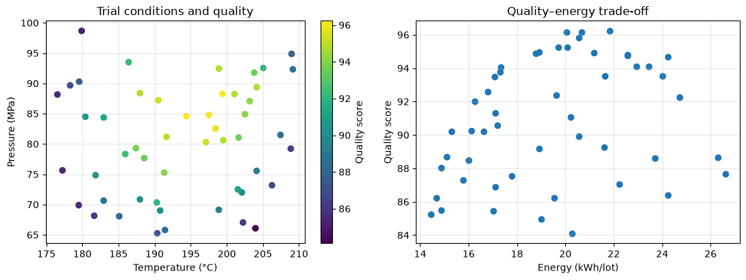
Standardize changes from baseline conditions as $x_1=(T-190)/10, x_2=(P-80)/10$. Quality response includes curvature, interactions, and measurement variation.

N=50
T=rng.uniform(175,210,N); P=rng.uniform(65,100,N); x1=(T-190)/10; x2=(P-80)/10
quality=96-2.8*(x1-.45)**2-1.9*(x2-.55)**2+.8*x1*x2-.2*x1**4+rng.normal(0,.45,N)
energy=18+2.4*x1+1.6*x2+.5*x1**2+rng.normal(0,.2,N)
trials=pd.DataFrame({"temperature_C":T,"pressure_MPa":P,"quality_score":quality,"energy_kWh":energy}).round(3)
display(trials.head()); display(trials.describe().round(2))
fig,ax=plt.subplots(1,2,figsize=(11,4.2)); s=ax[0].scatter(T,P,c=quality,cmap="viridis"); fig.colorbar(s,ax=ax[0],label="Quality score")
ax[0].set(title="Trial conditions and quality",xlabel="Temperature (°C)",ylabel="Pressure (MPa)"); ax[0].grid(True,alpha=.3)
ax[1].scatter(energy,quality); ax[1].set(title="Quality–energy trade-off",xlabel="Energy (kWh/lot)",ylabel="Quality score"); ax[1].grid(True,alpha=.3); plt.tight_layout(); plt.show()

	temperature_C	pressure_MPa	quality_score	energy_kWh
0	202.088	71.997	89.902	20.565
1	190.361	65.258	87.285	15.760
2	205.051	92.542	92.254	24.720
3	199.408	88.270	96.230	21.816
4	178.296	89.681	86.874	17.090

	temperature_C	pressure_MPa	quality_score	energy_kWh
count	50.00	50.00	50.00	50.00
mean	193.73	80.34	90.89	19.50
std	9.82	9.11	3.63	3.25
min	176.53	65.26	84.11	14.44
25%	186.05	72.13	87.76	17.03
50%	193.03	80.84	90.82	19.57
75%	202.20	88.23	94.11	21.77
max	209.15	98.67	96.23	26.60

No.041: What is Nonlinear Optimization?

Meaning in Practice

Process conditions require appropriate temperatures, and both excess and deficiency can degrade quality. Choose conditions that balance quality and cost from a curved response surface.

Approach to Analysis and Modeling

Operating losses are summed up as quality loss and energy burden, $f(x)=2.8(x_1-.45)^2+1.9(x_2-.55)^2-.8x_1x_2+.2x_1^4+.12(x_1+x_2)$.

Check with Python

def loss(x):
 a,b=x; return 2.8*(a-.45)**2+1.9*(b-.55)**2-.8*a*b+.2*a**4+.12*(a+b)
g=np.linspace(-1.5,2,150); X,Y=np.meshgrid(g,g); Z=np.vectorize(lambda a,b:loss([a,b]))(X,Y); r41=minimize(loss,[0,0],method="BFGS")
plt.contourf(190+10*X,80+10*Y,Z,25,cmap="viridis"); plt.colorbar(label="Operating loss"); plt.scatter(190+10*r41.x[0],80+10*r41.x[1],c="red",marker="*",s=180,label="Optimum")
plt.title("Nonlinear operating-loss surface"); plt.xlabel("Temperature (°C)"); plt.ylabel("Pressure (MPa)"); plt.grid(True,alpha=.3); plt.legend(); plt.tight_layout(); plt.show()
pd.Series({"temperature_C":190+10*r41.x[0],"pressure_MPa":80+10*r41.x[1],"minimum_loss":r41.fun,"success":r41.success})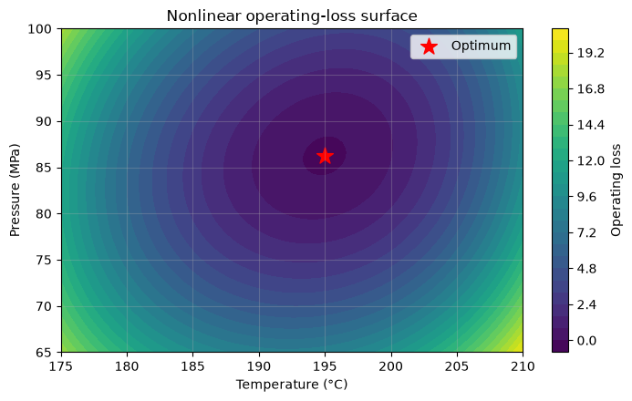

temperature_C    194.998253
pressure_MPa      86.236484
minimum_loss      -0.084816
success                True
dtype: object

Reading the results

The optimal point is in the valley of the response surface. The coefficient is converted to the same scale such as defective costs or electricity costs, and the basis is clearly provided.

No.042: What is a gradient?

Meaning in Practice

The gradient is the loss sensitivity when conditions are slightly adjusted, while the negative gradient represents the local improvement direction.

Approach to Analysis and Modeling

$\nabla f=(\partial f/\partial x_1,\partial f/\partial x_2)$。 The higher the absolute value, the greater the adjustment effect.

Check with Python

def grad(x):
 a,b=x; return np.array([5.6*(a-.45)-.8*b+.8*a**3+.12,3.8*(b-.55)-.8*a+.12])
pts=np.array([[-1,-.5],[0,0],[.8,.8],[1.5,1.2]])
pd.DataFrame([[190+10*a,80+10*b,loss([a,b]),*grad([a,b]),np.linalg.norm(grad([a,b]))] for a,b in pts],columns=["temperature_C","pressure_MPa","loss","grad_x1","grad_x2","gradient_norm"]).round(3)

	temperature_C	pressure_MPa	loss	grad_x1	grad_x2	gradient_norm
0	180.0	75.0	7.602	-8.40	-3.07	8.943
1	190.0	80.0	1.142	-2.40	-1.97	3.105
2	198.0	88.0	0.224	1.85	0.43	1.899
3	205.0	92.0	3.786	7.74	1.39	7.864

Reading the results

The code and size vary depending on the location. Zero gradient is a candidate point, and whether it is the minimum point is checked by curvature.

No.043: Slope Descent Method

Meaning in Practice

Move repeatedly toward improvement. If the learning rate is low, it is slow; if it is large, it jumps over valleys.

Approach to Analysis and Modeling

The update formula is $x^{(k+1)}=x^{(k)}-\alpha\nabla f(x^{(k)})$. Use a gradient norm for stopping.

Check with Python

def gd(x0,a,n=80):
 x=np.array(x0,dtype=float); h=[x.copy()]
 for _ in range(n):
  if np.linalg.norm(grad(x))<1e-7: break
  x-=a*grad(x); h.append(x.copy())
 return x,np.array(h)
rows=[]
for a in [.03,.12,.30]:
 x,h=gd([-1.2,1.5],a); v=[loss(z) for z in h]; plt.plot(v,label=f"alpha={a}"); rows.append([a,len(h)-1,v[-1],np.linalg.norm(grad(x))])
plt.title("Gradient descent convergence"); plt.xlabel("Iteration"); plt.ylabel("Operating loss"); plt.grid(True,alpha=.3); plt.legend(); plt.tight_layout(); plt.show()
pd.DataFrame(rows,columns=["learning_rate","iterations","final_loss","gradient_norm"]).round(6)

/var/folders/3y/fmw40k0x78xblvb3gkcyvy1h0000gn/T/ipykernel_25563/1166959326.py:2: RuntimeWarning: overflow encountered in scalar power
  a,b=x; return np.array([5.6*(a-.45)-.8*b+.8*a**3+.12,3.8*(b-.55)-.8*a+.12])
/var/folders/3y/fmw40k0x78xblvb3gkcyvy1h0000gn/T/ipykernel_25563/1702839514.py:5: RuntimeWarning: invalid value encountered in subtract
  x-=a*grad(x); h.append(x.copy())

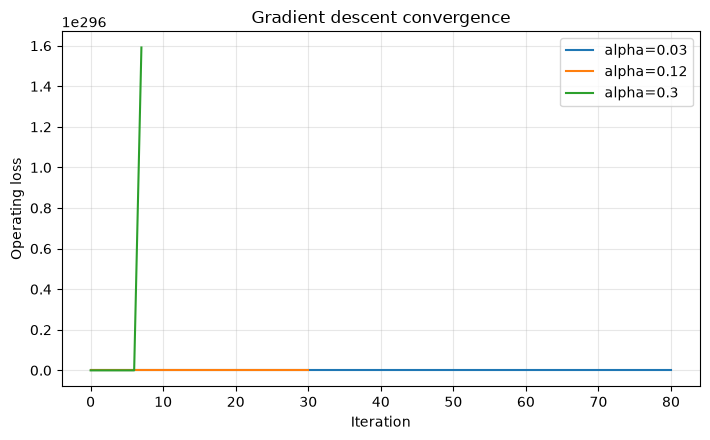
	learning_rate	iterations	final_loss	gradient_norm
0	0.03	80	-0.084816	0.000134
1	0.12	30	-0.084816	0.000000
2	0.30	80	NaN	NaN

Reading the results

The speed of convergence changes with your stride. Line search, scaling, and convergence history storage are practically important.

No.044: Newton’s Method

Meaning in Practice

Because it uses both slope and curvature, it is fast near the optimal point, but be mindful of the computational load of second-order derivatives.

Approach to Analysis and Modeling

$x^{(k+1)}=x^{(k)}-H^{-1}\nabla f$ using Hessian $H$. Solve the simultaneous equations instead of the inverse matrix.

Check with Python

def hess(x): return np.array([[5.6+2.4*x[0]**2,-.8],[-.8,3.8]])
x=np.array([-1.2,1.5]); rows=[]
for k in range(15):
 rows.append([k,*x,loss(x),np.linalg.norm(grad(x))])
 if np.linalg.norm(grad(x))<1e-10: break
 x-=np.linalg.solve(hess(x),grad(x))
pd.DataFrame(rows,columns=["iteration","x1","x2","loss","gradient_norm"]).round(8)

	iteration	x1	x2	loss	gradient_norm
0	0	-1.200000	1.500000	11.228470	1.260723e+01
1	1	0.005619	0.519604	0.615376	2.784218e+00
2	2	0.518210	0.627518	-0.083794	1.112897e-01
3	3	0.499894	0.623662	-0.084816	4.123200e-04
4	4	0.499825	0.623647	-0.084816	1.000000e-08
5	5	0.499825	0.623647	-0.084816	0.000000e+00

Reading the results

With minimal repetition, the gradient drops sharply. Comparisons are made based on the total computation time including differentiation, not the number of iterations.

No.045: Quasi-Newtonian Method

Meaning in Practice

Without implementing Hessian, we approximate curvature from gradient changes to achieve both accuracy and load.

Approach to Analysis and Modeling

BFGS sequentially updates the Hessian approximation based on movement and gradient differences.

Check with Python

rows=[]
for method in ["BFGS","CG"]:
 r=minimize(loss,[-1.2,1.5],jac=grad,method=method,options={"gtol":1e-9}); rows.append([method,r.success,r.nit,r.nfev,r.fun,190+10*r.x[0],80+10*r.x[1]])
pd.DataFrame(rows,columns=["method","success","iterations","function_evals","final_loss","temperature_C","pressure_MPa"]).round(6)

	method	success	iterations	function_evals	final_loss	temperature_C	pressure_MPa
0	BFGS	True	9	10	-0.084816	194.998255	86.236475
1	CG	True	8	19	-0.084816	194.998255	86.236475

Reading the results

Not only the success flag, but also the final gradient and the number of evaluations are recorded.

No.046：L-BFGS

Meaning in Practice

For problems with many variables, L-BFGS, which only has the most recent history, consumes memory.

Approach to Analysis and Modeling

Penalties are imposed simultaneously for discrepancies between the individual targets of the 100 processes and sudden changes in adjacent processes. L-BFGS-B can handle both upper and lower limits.

Check with Python

q=100; target=.5+.25*np.sin(np.linspace(0,4*np.pi,q))
def lf(z): return np.sum((z-target)**2)+.4*np.sum(np.diff(z)**2)+.02*np.sum(z**4)
def lg(z):
 g=2*(z-target)+.08*z**3; d=np.diff(z); g[:-1]-=.8*d; g[1:]+=.8*d; return g
r46=minimize(lf,np.zeros(q),jac=lg,method="L-BFGS-B",bounds=[(-1,1)]*q)
plt.plot(target,"--",label="Individual target"); plt.plot(r46.x,label="Optimized setting"); plt.title("L-BFGS-B for 100 process settings"); plt.xlabel("Process index"); plt.ylabel("Scaled setting"); plt.grid(True,alpha=.3); plt.legend(); plt.tight_layout(); plt.show()
pd.Series({"success":r46.success,"iterations":r46.nit,"final_loss":r46.fun})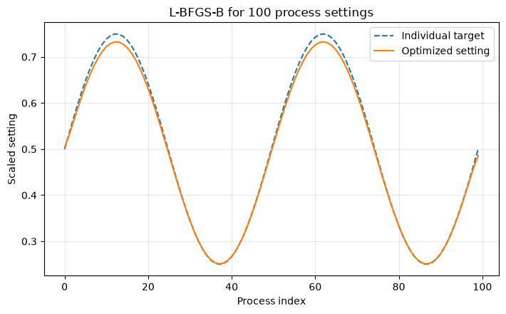

success           True
iterations           8
final_loss    0.231526
dtype: object

Reading the results

We kept track of individual goals while preventing sudden changes. Memory, computation time, and recalculation frequency are also required.

No.047: Lagrange Indefinite Multiplier Method

Meaning in Practice

If the total equipment load is constant, the best point on the constraint boundary is sought.

Approach to Analysis and Modeling

$q=(x_1-1)^2+2(x_2-1)^2$, solve the stop conditions for $\mathcal L=q+\lambda h$ as $h=x_1+x_2-1=0$.

Check with Python

A=np.array([[2,0,1],[0,4,1],[1,1,0]],float); b=np.array([2,4,1],float); a,bv,lam=np.linalg.solve(A,b)
pd.Series({"x1":a,"x2":bv,"lambda":lam,"constraint_residual":a+bv-1,"quality_loss":(a-1)**2+2*(bv-1)**2}).round(6)

x1                     0.333333
x2                     0.666667
lambda                 1.333333
constraint_residual    0.000000
quality_loss           0.666667
dtype: float64

Reading the results

The multiplier is the local value of constraint relaxation. Since the code depends on the definition, check the change in the desired value when changing the right side.

No.048: KKT Conditions

Meaning in Practice

Identify which constraints restrict solutions, and use these as materials for facility upgrades and standards revisions.

Approach to Analysis and Modeling

Under $g_i(x)\le0$, check the principal/dual feasibility, retention conditions, and complementarity $\mu_i g_i=0$.

Check with Python

def ko(x): return (x[0]-1)**2+(x[1]-1)**2
r48=minimize(ko,[.2,.2],method="SLSQP",constraints=[{"type":"ineq","fun":lambda x:1.2-x.sum()}]); x=r48.x; mu=2*(1-x[0]); gv=x.sum()-1.2
st=np.array([2*(x[0]-1)+mu,2*(x[1]-1)+mu])
pd.Series({"x1":x[0],"x2":x[1],"g(x)<=0":gv,"mu>=0":mu,"stationarity_norm":np.linalg.norm(st),"complementarity":mu*gv}).round(8)

x1                   0.6
x2                   0.6
g(x)<=0              0.0
mu>=0                0.8
stationarity_norm    0.0
complementarity      0.0
dtype: float64

Reading the results

The limitation is activity, and the KKT residual is almost zero. Active constraints and multipliers indicate the value of additional abilities.

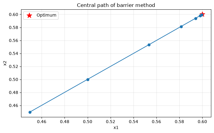
No.049: Interior Point Method

Meaning in Practice

Proceed inside inequality constraints and approach the solution at the boundary.

Approach to Analysis and Modeling

$x_1,x_2>0$, $x_1+x_2<1.2$ A logarithmic barrier is added to gradually weaken it.

Check with Python

def barrier(x,t):
 s=1.2-x.sum()
 return np.inf if min(x)<=0 or s<=0 else ko(x)-(np.log(x[0])+np.log(x[1])+np.log(s))/t
x=np.array([.3,.3]); path=[]
for t in [1,3,10,30,100,300,1000]:
 r=minimize(lambda z:barrier(z,t),x,method="Nelder-Mead"); x=r.x; path.append([t,*x,1.2-x.sum(),ko(x)])
df=pd.DataFrame(path,columns=["t","x1","x2","slack","objective"]); display(df.round(6))
plt.plot(df.x1,df.x2,marker="o"); plt.scatter(.6,.6,c="red",marker="*",s=160,label="Optimum"); plt.title("Central path of barrier method"); plt.xlabel("x1"); plt.ylabel("x2"); plt.grid(True,alpha=.3); plt.legend(); plt.tight_layout(); plt.show()

	t	x1	x2	slack	objective
0	1	0.449621	0.449651	0.300727	0.605800
1	3	0.499973	0.500000	0.200026	0.500026
2	10	0.553489	0.553382	0.093129	0.398840
3	30	0.581397	0.581342	0.037261	0.350503
4	100	0.594008	0.593921	0.012071	0.329730
5	300	0.597956	0.597923	0.004121	0.323306
6	1000	0.599346	0.599408	0.001245	0.320997

Reading the results

Weakening the barrier reduces the constraint margin. Return the allowable error to physical units and confirm the safety margin.

No.050: Nonlinear Optimization and Machine Learning

Meaning in Practice

Connecting the predictive model to the next driving conditions for decision-making.

Approach to Analysis and Modeling

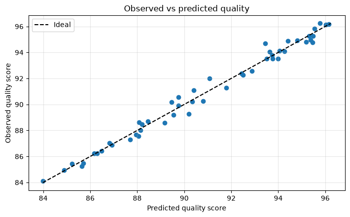
From the prototype, you will learn nonlinear regression $\hat y(x)$ and solve $\min\{-\hat y(x)+\rho E(x)\}$ within the scope of the prototype.

Check with Python

def feat(a,b):
 a,b=np.asarray(a),np.asarray(b); return np.column_stack([np.ones_like(a),a,b,a*a,a*b,b*b,a**3,a**4])
coef,*_=np.linalg.lstsq(feat(x1,x2),quality,rcond=None); pred=feat(x1,x2)@coef; rmse=np.sqrt(np.mean((quality-pred)**2))
def pq(x): return float((feat([x[0]],[x[1]])@coef).item())
def dl(x): return -pq(x)+.12*(18+2.4*x[0]+1.6*x[1]+.5*x[0]**2)
r50=minimize(dl,[0,0],method="L-BFGS-B",bounds=[(x1.min(),x1.max()),(x2.min(),x2.max())])
display(pd.Series({"training_RMSE":rmse,"recommended_temperature_C":190+10*r50.x[0],"recommended_pressure_MPa":80+10*r50.x[1],"predicted_quality":pq(r50.x),"success":r50.success}).round(4))
plt.scatter(pred,quality); lo=min(pred.min(),quality.min()); hi=max(pred.max(),quality.max()); plt.plot([lo,hi],[lo,hi],"--",color="black",label="Ideal"); plt.title("Observed vs predicted quality"); plt.xlabel("Predicted quality score"); plt.ylabel("Observed quality score"); plt.grid(True,alpha=.3); plt.legend(); plt.tight_layout(); plt.show()

training_RMSE                   0.43307
recommended_temperature_C    194.965778
recommended_pressure_MPa      86.175973
predicted_quality             96.258864
success                            True
dtype: object

Reading the results

Within learning, RMSE alone is not enough. Verification data, prediction intervals, extrapolation prevention, and verification tests under recommended conditions are required.

Practical Implications Seen Through Target Exercise

• The objective coefficient requires evidence such as defective costs, electricity costs, and delivery time impacts.
• Variable scaling helps with convergence and managing tolerance of error.
• KKT multipliers and activation constraints can be used as priorities for equipment expansion.
• Stores initial values, convergence history, constraint residuals, and recalculation conditions.
• Prediction accuracy and optimization results are verified separately to prevent extrapolation.

What is necessary for practical implementation

Points of Contention	confirmation item	deliverable
KPI	Conversion of quality, cost, and delivery time	Objective Function Definition Book
restriction	Equipment limits, specifications, safety margins	List of Constraints and Rationale
Data	Measurement system, missing measurements, test scope	Data dictionary
verification	Current Comparison, Sensitivity, Extrapolation	Confirmation Test Plan
Utilization	Approval, recalculation, and handling abnormalities	SOP and Monitoring Metrics

Start with decision support where people check recommended values, then expand automation while verifying effectiveness and safety.

Conclusion

We reviewed everything from formulating nonlinear responses to solutions using gradients and curvature, checking constrained solutions, and recommending conditions using machine learning. Optimization is not just about calculation; it is a decision-making process that clarifies objectives and constraints, sharing areas for improvement and risks.

Consultations for Corporations

At Mathematical Laboratory, we support problem organization, PoC, and operational design for manufacturing condition optimization, production planning, simulation, and the integration of forecasting and optimization.

📩 Contact Us: surikobo.co.jp/contact
Please feel free to consult us first.