Turning the “Usual” in Manufacturing Sites into Decision-Making: 10 Key Exercises on the Basics of Anomaly Detection

In this article, we use a fictional precision parts factory as a subject to teach the basic concepts of anomaly detection in Judgments on quality, equipment maintenance, and production management. Through No.001 to No.010, we organize everything from defining anomalies, selecting data and methods, to conducting PoC (proof of concept) as a single flow.

This “100 Anomaly Detection Exercises” consists of 10 chapters: basics, preprocessing, statistics, time series, sensors, machine learning, multivariates, deep learning, evaluation and alerts, and practical operations. The goal is not to memorize algorithms, but to acquire The ability to turn detection results into actions such as inspection, stopping, maintenance, and improvement. This article serves as Chapter 1, serving as the entry point.

[!NOTE] This material is a notebook previously used by Surikoubo (or personally by the representative, Kazuyama), and has been reconstructed, edited, and published with the company’s permission.
All data listed is fictional and has no relation whatsoever to real companies, factories, or figures.

Introduction: Practical Challenges in Manufacturing Covered in This Article

In manufacturing sites, various “differences” such as rising temperatures, increased vibration, dimensional deviations, and yield decreases occur. However, stopping equipment just because the value is rare is considered over-response, and missing changes with significant operational impact can lead to defect outages or sudden shutdowns.

The question addressed in this article is What are called anomalies, what data are captured, and who responds how?. We emphasize not only analysts but also manufacturing, quality, maintenance, and production management sharing a common language.

Common situations on site

• Values exceeding the management limit are notified, but there are many alerts that cannot be fully verified.
• There are few normal and abnormal labels, and the failure history and sensor log times are not aligned.
• Statistically, it’s rare, but since it’s just been replaced, the site has values that are expected
• Even if a single point is normal, a series of tiny changes can be a sign of malfunction
• Although model accuracy has been reported, the boundaries of responsibility for stop decisions and maintenance instructions remain undecided

Why is this issue so difficult to judge?

“Abnormalities” are not uniquely determined by data alone. It is necessary to simultaneously consider the frequency of occurrence, process conditions, the magnitude of losses, and the actions that can be taken after detection. Additionally, since fewer failures are desirable, there is a contradiction in that it is inherently difficult to gather abnormal cases necessary for supervised learning.

If we $s(\mathbf{x})$ the abnormal score representing statistical rarity and the notification threshold $\tau$, the basic form is as follows.

$$\text{alert}(\mathbf{x}) = \mathbb{1}\left[s(\mathbf{x}) > \tau\right]$$

However, $\tau$ is determined not only based on mathematics, but also on missed losses, man-hours spent in handling false alarms, safety standards, and the number of cases that can be processed per day.

Overview of Exercise covered this time

No.	Theme	Connecting to decision-making
001	What is Anomaly Detection?	Defining Surveillance to Action
002	Abnormal values, outliers, and abnormal conditions	Do not confuse inspection targets with data corrections
003	Statistical and operational anomalies	Combining on-site rules and statistics
004	With and without teachers	Choose your method based on label maturity
005	Point, context, and set anomalies	Consider time and continuity
006	Representative Data	Designing data granularity and keys
007	Applications in Manufacturing	Expanding into Quality, Production, and Safety
008	Utilization for equipment maintenance	Turning Signs into Conservation Priorities
009	Utilization of Business Data	Detecting signs outside the sensor
010	How the Project Proceeds	Designing from PoC to Operation

Preparing the Python environment

numpy, pandas, and matplotlib are used exclusively. Fix the random number seed so you can reproduce the same result. To avoid differences in Japanese fonts due to environmental factors, the graphs are displayed in English, and the following markdown explains the operational meanings in Japanese.

import platform
import numpy as np
import pandas as pd
import matplotlib
import matplotlib.pyplot as plt
from IPython.display import display

SEED = 42
rng = np.random.default_rng(SEED)
plt.rcParams.update({"figure.figsize": (10, 4.5), "axes.grid": True})

print("Python     :", platform.python_version())
print("NumPy      :", np.__version__)
print("pandas     :", pd.__version__)
print("matplotlib :", matplotlib.__version__)

Python     : 3.13.1
NumPy      : 2.5.1
pandas     : 3.0.3
matplotlib : 3.11.0

Creation of Fictional Data

We create logs for two days of processing equipment M-01, which operates every 5 minutes. In addition to temperature, vibration, spindle load, and product dimensions, it includes shift, type, setup status, and maintenance labels. Intentionally embedded single spikes, temperature issues that only occur during night shifts, continuous increases in vibration, and sensor defects.

n = 576
ts = pd.date_range("2026-04-01", periods=n, freq="5min")
t = np.arange(n)
shift = np.where((ts.hour >= 8) & (ts.hour < 20), "day", "night")
product = np.where((t // 72) % 2 == 0, "A", "B")
setup = (t % 72 < 5)

temperature = 68 + 2.2 * np.sin(2 * np.pi * t / 288) + rng.normal(0, 0.7, n)
vibration = 1.8 + 0.12 * np.sin(2 * np.pi * t / 60) + rng.normal(0, 0.08, n)
load = 62 + np.where(product == "B", 7, 0) + rng.normal(0, 3.0, n)
dimension = 20 + np.where(product == "B", 0.015, 0) + rng.normal(0, 0.012, n)

temperature[430] = 82.0                     # Single point abnormality
temperature[40] = 74.5                      # Problems in the context of night shifts
vibration[300:312] += np.linspace(0.3, 1.5, 12)  # Cluster anomalies and warning signs of failure
dimension[145] = 20.11                      # Deviation from Specifications
temperature[210] = np.nan                   # communication loss
maintenance_label = np.zeros(n, dtype=int)
maintenance_label[300:312] = 1

df = pd.DataFrame({
    "timestamp": ts, "equipment": "M-01", "shift": shift,
    "product": product, "setup": setup, "temperature_c": temperature,
    "vibration_mm_s": vibration, "spindle_load_pct": load,
    "dimension_mm": dimension, "maintenance_label": maintenance_label,
})
display(df.head())
print(f"rows={len(df):,}, period={df.timestamp.min()} - {df.timestamp.max()}")

	timestamp	equipment	shift	product	setup	temperature_c	vibration_mm_s	spindle_load_pct	dimension_mm	maintenance_label
0	2026-04-01 00:00:00	M-01	night	A	True	68.213302	1.906895	62.817936	20.000879	0
1	2026-04-01 00:05:00	M-01	night	A	True	67.320004	1.912379	60.315551	20.000450	0
2	2026-04-01 00:10:00	M-01	night	A	True	68.621278	1.804748	64.093451	19.998910	0
3	2026-04-01 00:15:00	M-01	night	A	True	68.802282	1.866158	62.331839	19.999630	0
4	2026-04-01 00:20:00	M-01	night	A	True	66.826018	1.656015	62.004020	19.997427	0

rows=576, period=2026-04-01 00:00:00 - 2026-04-02 23:55:00

No.001: Organizing What Anomaly Detection Means

Meaning in Practice

Anomaly detection is not a “technique for searching for abnormal values,” but rather a mechanism that detects deviations from normal operating patterns early and encourages actions such as confirmation, adjustment, and maintenance. Operational value is only realized when the detection target, timing of detection, person in charge, and primary response are defined.

Approach to Analysis and Modeling

Here, the normal temperature range is summarized using an average $\mu$ and standard deviation $\sigma$, with points exceeding $\mu+3\sigma$ as candidates. This is not a confirmation of abnormalities but a primary screening to narrow down the scope of the investigation. As a rule, mean and standard deviation are estimated from the reference period excluding known anomalies and defects.

Check with Python

baseline = df.loc[:287, "temperature_c"].dropna()
mu, sigma = baseline.mean(), baseline.std()
threshold = mu + 3 * sigma
candidate = df["temperature_c"] > threshold

fig, ax = plt.subplots()
ax.plot(df["timestamp"], df["temperature_c"], label="Temperature", linewidth=1)
ax.axhline(threshold, color="tab:red", linestyle="--", label="Baseline mean + 3 SD")
ax.scatter(df.loc[candidate, "timestamp"], df.loc[candidate, "temperature_c"], color="tab:red", label="Candidates", zorder=3)
ax.set_title("Temperature anomaly screening")
ax.set_xlabel("Timestamp"); ax.set_ylabel("Temperature (C)")
ax.grid(True, alpha=0.3); ax.legend(); fig.tight_layout()
plt.show()
print(f"threshold={threshold:.2f} C, candidates={candidate.sum()}")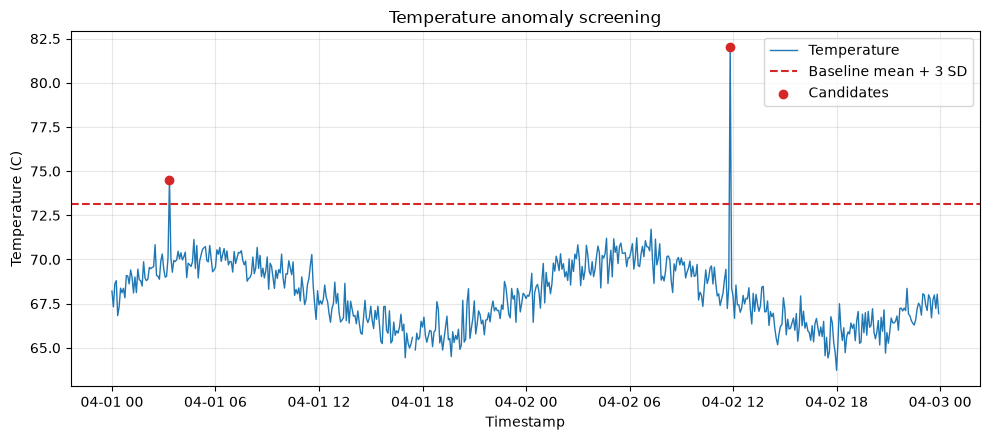

threshold=73.14 C, candidates=2

Reading the results

Multiple threshold exceedances are extracted, but not all are subject to stopping. We check the time, variety, schedule, and other sensors together to determine the severity. The division of roles in The model’s output is a judgment material, not a judgment itself is important.

No.002: Understanding the Differences Between Outliers, Outliers, and Abnormal States

Meaning in Practice

• abnormal value: Values questionable in validity, including errors in measurement, input, or communication
• outlier: Values statistically diverged from other observations. Sometimes the measurements are correct
• abnormal state: Undesirable conditions in equipment or processes. It holds even if there is no single outlier

If these are confused, failure signs may be erased as missing or unnecessary maintenance may be performed due to communication errors.

Approach to Analysis and Modeling

First, physical validity and deficiencies are examined, then statistical anomalies are extracted, and finally, the state is evaluated using operational rules and multiple variables. Data quality flags and equipment status flags are managed in separate columns.

Check with Python

check = df.copy()
check["data_quality_issue"] = check["temperature_c"].isna() | ~check["temperature_c"].between(0, 150)
q1, q3 = check["dimension_mm"].quantile([0.25, 0.75])
iqr = q3 - q1
check["statistical_outlier"] = ~check["dimension_mm"].between(q1 - 1.5 * iqr, q3 + 1.5 * iqr)
check["abnormal_state"] = (check["vibration_mm_s"].rolling(6, min_periods=6).mean() > 2.35)

summary = pd.Series({
    "data_quality_issue": int(check["data_quality_issue"].sum()),
    "statistical_outlier": int(check["statistical_outlier"].sum()),
    "abnormal_state": int(check["abnormal_state"].sum()),
}, name="count").to_frame()
display(summary)
display(check.loc[check[["data_quality_issue", "statistical_outlier", "abnormal_state"]].any(axis=1),
                  ["timestamp", "temperature_c", "dimension_mm", "vibration_mm_s",
                   "data_quality_issue", "statistical_outlier", "abnormal_state"]].head(10))

	count
data_quality_issue	1
statistical_outlier	2
abnormal_state	10

	timestamp	temperature_c	dimension_mm	vibration_mm_s	data_quality_issue	statistical_outlier	abnormal_state
145	2026-04-01 12:05:00	67.661257	20.110000	1.950242	False	True	False
187	2026-04-01 15:35:00	65.368694	19.963428	1.931248	False	True	False
210	2026-04-01 17:30:00	NaN	19.991873	1.803537	True	False	False
305	2026-04-02 01:25:00	68.060335	19.995237	2.781267	False	False	True
306	2026-04-02 01:30:00	68.607784	20.001365	2.736191	False	False	True
307	2026-04-02 01:35:00	69.796074	20.008842	2.850174	False	False	True
308	2026-04-02 01:40:00	69.337619	19.994449	2.974439	False	False	True
309	2026-04-02 01:45:00	70.185653	20.011959	3.202014	False	False	True
310	2026-04-02 01:50:00	69.840035	19.988076	3.394428	False	False	True
311	2026-04-02 01:55:00	69.365536	20.003535	3.375118	False	False	True

Reading the results

Missing items, dimensional misalignments, and persistent abnormal vibrations appear as separate cases. For defects, check instrumentation and communication; for dimensional deviations, quality isolation; and for ongoing vibrations, maintenance inspections—designing with different targets for each flag is necessary.

No.003: Distinguishing Statistical Anomalies from Operational Anomalies

Meaning in Practice

Statistical anomalies mean “rare,” while operational anomalies mean “issues with standards, safety, delivery times, or costs.” While there are rare and acceptable prototyping conditions, statistically common ones that slightly deviate from customer standards are nonconforming.

Approach to Analysis and Modeling

Statistical rules and operational rules are evaluated separately, and overlaps are checked. Here, we compare the temperature Z-score $z=(x-\mu)/\sigma$ with the work rule of a night shift upper limit of 72°C.

Check with Python

temp_mean = df["temperature_c"].mean()
temp_std = df["temperature_c"].std()
df["statistical_anomaly"] = ((df["temperature_c"] - temp_mean) / temp_std).abs() > 3
df["business_anomaly"] = (df["shift"] == "night") & (df["temperature_c"] > 72)

comparison = pd.crosstab(df["statistical_anomaly"], df["business_anomaly"],
                         rownames=["Statistical"], colnames=["Business"])
display(comparison)
display(df.loc[df["statistical_anomaly"] | df["business_anomaly"],
               ["timestamp", "shift", "temperature_c", "statistical_anomaly", "business_anomaly"]])

Business	False	True
Statistical
False	574	0
True	1	1

	timestamp	shift	temperature_c	statistical_anomaly	business_anomaly
40	2026-04-01 03:20:00	night	74.5	True	True
430	2026-04-02 11:50:00	day	82.0	True	False

Reading the results

The two types of flags do not match perfectly. Statistical models alone may overlook night-shift specific operating conditions, while business rules alone may miss unknown extremes. Using both together and including the reason code with the notification makes it easier for the site to verify.

No.004: Comparing Supervised and Unsupervised Anomaly Detection

Meaning in Practice

Supervised methods learn from past fault labels and can easily reproduce known anomalies with high accuracy, but label creation and addressing unknown failures remain challenges. Unsupervised methods can find unusual patterns without labels, but extraction results are not necessarily business-important.

Approach to Analysis and Modeling

Method selection is not based on trends, but on label volume, label reliability, importance of unknown anomalies, and accountability. Here, candidate methods are compared in decision tables and conservation label biases are also checked.

Check with Python

method_table = pd.DataFrame({
    "approach": ["Supervised", "Unsupervised", "Rule + score hybrid"],
    "label_requirement": ["Many reliable labels", "Not required", "A few reviewed cases"],
    "strength": ["Known failure recognition", "Unknown pattern discovery", "Explainability and gradual rollout"],
    "main_risk": ["Misses unseen failure modes", "Many irrelevant alerts", "Rules require maintenance"],
    "recommended_phase": ["Mature operation", "Early exploration", "PoC to early operation"],
})
display(method_table)
label_counts = df["maintenance_label"].value_counts().rename(index={0: "normal", 1: "anomaly"})
display(label_counts.to_frame("records"))
print(f"anomaly prevalence={df['maintenance_label'].mean():.2%}")

	approach	label_requirement	strength	main_risk	recommended_phase
0	Supervised	Many reliable labels	Known failure recognition	Misses unseen failure modes	Mature operation
1	Unsupervised	Not required	Unknown pattern discovery	Many irrelevant alerts	Early exploration
2	Rule + score hybrid	A few reviewed cases	Explainability and gradual rollout	Rules require maintenance	PoC to early operation

	records
maintenance_label
normal	564
anomaly	12

anomaly prevalence=2.08%

Reading the results

Abnormal labels make up only a small portion of the total and are unbalanced. At this stage, a hybrid operation is realistic by presenting candidates based on unsupervised scores and on-site rules, and accumulating confirmation results from maintenance personnel. The accumulated reviews can be used for future supervised learning.

No.005: Understanding Point Anomaly, Contextual Anomaly, and Set Anomaly

Meaning in Practice

Point anomalies are extremes from single observations; contextual anomalies are values that are unnatural when considering shifts or varieties; and ensemble anomalies are states where individual values are minor but are continuous or unnatural as a group. Signs in manufacturing often appear as collective anomalies.

Approach to Analysis and Modeling

For point anomalies, use the global threshold; for contextual anomalies, use conditional criteria; for set anomalies, use moving averages or consecutive counts. If you treat rows independently regardless of chronological order, the information about set anomalies is lost.

Check with Python

point_flag = df["temperature_c"] > 80
context_flag = (df["shift"] == "night") & (df["temperature_c"] > 72)
rolling_vib = df["vibration_mm_s"].rolling(6, min_periods=6).mean()
collective_flag = rolling_vib > 2.35

fig, axes = plt.subplots(2, 1, figsize=(10, 7), sharex=True)
axes[0].plot(df["timestamp"], df["temperature_c"], linewidth=1)
axes[0].scatter(df.loc[point_flag | context_flag, "timestamp"],
                df.loc[point_flag | context_flag, "temperature_c"], color="tab:red")
axes[0].set_title("Point and contextual anomalies"); axes[0].set_ylabel("Temperature (C)")
axes[0].grid(True, alpha=0.3)
axes[1].plot(df["timestamp"], rolling_vib, label="6-point rolling mean")
axes[1].axhline(2.35, color="tab:red", linestyle="--", label="Collective threshold")
axes[1].fill_between(df["timestamp"], 0, rolling_vib, where=collective_flag, color="tab:red", alpha=0.25)
axes[1].set_title("Collective anomaly in vibration"); axes[1].set_xlabel("Timestamp")
axes[1].set_ylabel("Vibration (mm/s)"); axes[1].grid(True, alpha=0.3); axes[1].legend()
fig.tight_layout(); plt.show()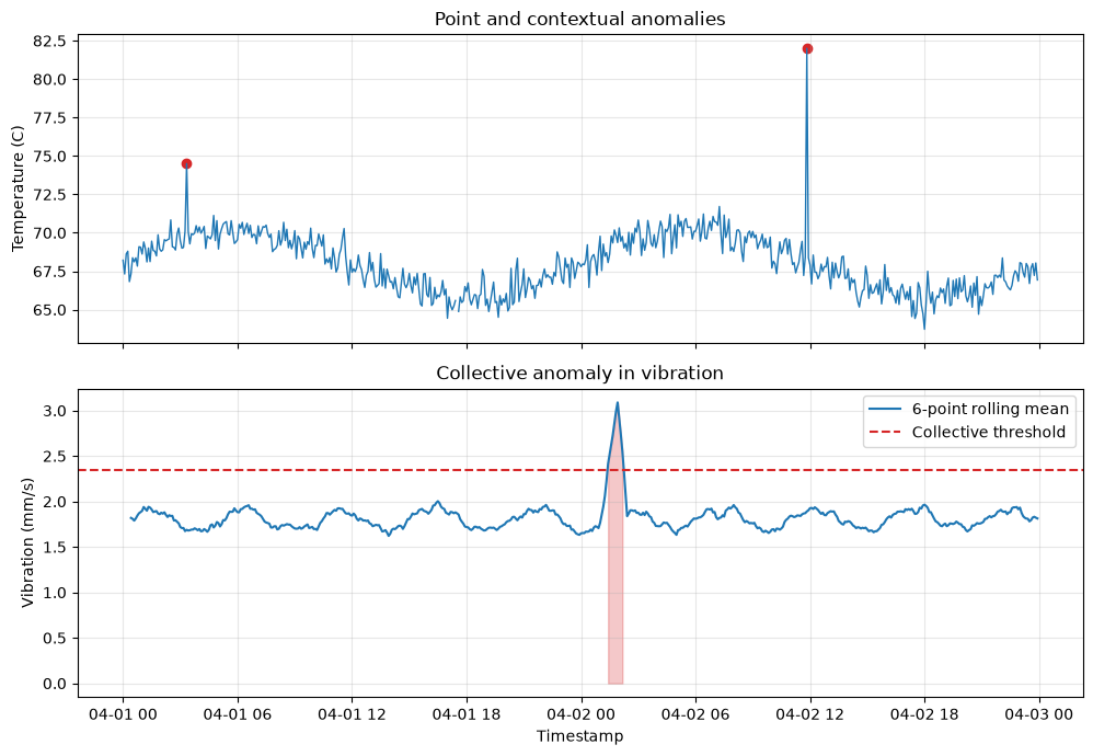

Reading the results

Temperature spikes should be checked immediately; temperature increases under night shift conditions should be checked under operating conditions; continuous vibration increases should be considered for early planned maintenance. Even with the same “anomaly,” the required timeline and actions differ, so include the type in the notification.

No.006: Organizing representative data handled in anomaly detection

Meaning in Practice

Abnormality detection is not complete by sensors alone. By connecting inspection, operation, alarms, maintenance, working conditions, environment, and order placement, you can identify potential causes and operational impacts.

Approach to Analysis and Modeling

What matters more than the data volume is the meaning of the connection keys for equipment ID, model number, lot, time, granularity, acquisition delays, and missing data. First, create a data ledger and clarify what each row represents.

Check with Python

data_catalog = pd.DataFrame([
    ["Sensor", "5 minutes", "equipment + timestamp", "Temperature, vibration", "Condition monitoring"],
    ["Inspection", "product", "lot + serial", "Dimension, pass/fail", "Quality containment"],
    ["Production", "lot", "equipment + lot", "Count, cycle time", "Loss detection"],
    ["Maintenance", "work order", "equipment + work time", "Part, symptom, action", "Cause validation"],
    ["Master", "revision", "equipment/product ID", "Spec, location, model", "Context enrichment"],
], columns=["data_type", "grain", "join_key", "examples", "decision_use"])
display(data_catalog)
quality = df.isna().sum().to_frame("missing_count")
quality["missing_rate"] = df.isna().mean()
display(quality.query("missing_count > 0"))

	data_type	grain	join_key	examples	decision_use
0	Sensor	5 minutes	equipment + timestamp	Temperature, vibration	Condition monitoring
1	Inspection	product	lot + serial	Dimension, pass/fail	Quality containment
2	Production	lot	equipment + lot	Count, cycle time	Loss detection
3	Maintenance	work order	equipment + work time	Part, symptom, action	Cause validation
4	Master	revision	equipment/product ID	Spec, location, model	Context enrichment

	missing_count	missing_rate
temperature_c	1	0.001736

Reading the results

There is also a missing temperature in this log. If you fill in the missing point at zero, it creates a false sharp drop, so you should monitor it separately as a communication outage. In production, if you first establish the equipment ID system and time synchronization, you can greatly reduce rework in the analysis.

No.007: Organizing Examples of Anomaly Detection Applications in Manufacturing

Meaning in Practice

The applications are not limited to predictive maintenance. It covers areas where decision-making and losses can be defined, such as quality anomalies, cycle time delays, degraded energy intensity, and safety deviations.

Approach to Analysis and Modeling

Candidate themes are evaluated based on annual loss, detectability, post-detection feasibility, and data readiness. Themes that are somewhat simple but can be quickly moved on-site may find it easier to add value than themes that cannot be handled even with high accuracy.

Check with Python

use_cases = pd.DataFrame({
    "use_case": ["Quality drift", "Bearing degradation", "Cycle-time delay", "Energy loss"],
    "annual_loss_mjpy": [24, 40, 18, 12],
    "detectability": [4, 3, 4, 3],
    "actionability": [5, 4, 3, 4],
    "data_readiness": [5, 3, 4, 2],
})
use_cases["priority_score"] = (
    0.4 * use_cases["annual_loss_mjpy"] / use_cases["annual_loss_mjpy"].max() * 5
    + 0.2 * use_cases["detectability"]
    + 0.25 * use_cases["actionability"]
    + 0.15 * use_cases["data_readiness"]
)
display(use_cases.sort_values("priority_score", ascending=False).round(2))

fig, ax = plt.subplots()
ax.bar(use_cases["use_case"], use_cases["priority_score"], color="tab:blue")
ax.set_title("Anomaly-detection use-case priority")
ax.set_xlabel("Use case"); ax.set_ylabel("Priority score")
ax.grid(True, axis="y", alpha=0.3); ax.tick_params(axis="x", rotation=15); fig.tight_layout()
plt.show()

	use_case	annual_loss_mjpy	detectability	actionability	data_readiness	priority_score
1	Bearing degradation	40	3	4	3	4.05
0	Quality drift	24	4	5	5	4.00
2	Cycle-time delay	18	4	3	4	3.05
3	Energy loss	12	3	4	2	2.50

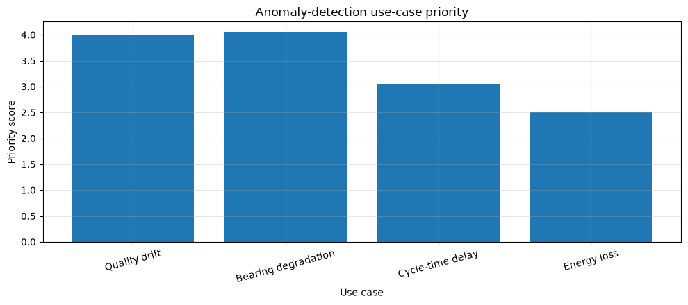
Reading the results

In hypothetical evaluations, quality drift is the top priority. This is not only because of annual losses, but also because testing data is complete, and actions such as isolation and adjustment of conditions are clear. Weights are agreed upon according to management policies, and sensitivity analysis is also conducted.

No.008: Organizing Examples of Abnormality Detection Applications in Equipment Maintenance

Meaning in Practice

In equipment maintenance, abnormality detection is not only used to “guess faults” but also to determine the inspection order and timing of inspections. Priority is determined by considering sudden downtime losses, parts delivery times, and safety risks.

Approach to Analysis and Modeling

Deviations from the vibration reference value are considered a simplified risk score, and only if the deviation from the baseline values is a candidate for inspection. To suppress single-source noise, it is important in practice to establish continuity and hysteresis.

Check with Python

vib_base = df.loc[:287, "vibration_mm_s"]
vib_z = (df["vibration_mm_s"] - vib_base.mean()) / vib_base.std()
df["maintenance_risk"] = vib_z.clip(lower=0)
df["inspection_candidate"] = df["maintenance_risk"].rolling(3, min_periods=3).min() > 3

top_risk = df.nlargest(8, "maintenance_risk")[
    ["timestamp", "vibration_mm_s", "maintenance_risk", "inspection_candidate"]
]
display(top_risk.round(2))
print("first inspection candidate:",
      df.loc[df["inspection_candidate"], "timestamp"].min())

/var/folders/3y/fmw40k0x78xblvb3gkcyvy1h0000gn/T/ipykernel_19197/885776230.py:9: UserWarning: obj.round has no effect with datetime, timedelta, or period dtypes. Use obj.dt.round(...) instead.
  display(top_risk.round(2))

	timestamp	vibration_mm_s	maintenance_risk	inspection_candidate
310	2026-04-02 01:50:00	3.39	13.49	True
311	2026-04-02 01:55:00	3.38	13.33	True
309	2026-04-02 01:45:00	3.20	11.86	True
308	2026-04-02 01:40:00	2.97	9.94	True
307	2026-04-02 01:35:00	2.85	8.89	True
305	2026-04-02 01:25:00	2.78	8.30	True
306	2026-04-02 01:30:00	2.74	7.92	True
304	2026-04-02 01:20:00	2.60	6.80	True

first inspection candidate: 2026-04-02 01:15:00

Reading the results

Under continuous conditions, inspection candidates will rise midway through the vibration rise. In actual operation, the suspension period is combined with spare parts inventory, and production planning, and is divided into “stop now,” “inspect at the next stop,” and “monitor the progress.”

No.009: Organizing Examples of Anomaly Detection in Business Data

Meaning in Practice

Anomalies also appear in business data such as daily reports, actual labor hours, inventory, purchasing, delivery dates, and inspection numbers. Even without equipment logs, you can quickly identify deterioration in yield, input stoppages, and process delays.

Approach to Analysis and Modeling

It aggregates daily production and defect counts, and monitors defect rates and data integrity. Since the rate on days with fewer transactions fluctuates easily, the denominator is also displayed simultaneously. You also need context such as business calendars, holidays, and inventory days.

Check with Python

daily = pd.DataFrame({
    "date": pd.date_range("2026-04-01", periods=14, freq="D"),
    "production_qty": rng.integers(900, 1100, 14),
    "defect_qty": rng.poisson(11, 14),
    "report_rows": rng.integers(18, 23, 14),
})
daily.loc[8, "defect_qty"] = 46
daily.loc[11, "report_rows"] = 4
daily["defect_rate"] = daily["defect_qty"] / daily["production_qty"]
daily["quality_alert"] = daily["defect_rate"] > 0.025
daily["data_delay_alert"] = daily["report_rows"] < 15
display(daily.loc[daily["quality_alert"] | daily["data_delay_alert"]].round(4))

fig, ax = plt.subplots()
ax.plot(daily["date"], daily["defect_rate"] * 100, marker="o")
ax.axhline(2.5, color="tab:red", linestyle="--", label="Review threshold")
ax.set_title("Daily defect-rate monitoring")
ax.set_xlabel("Date"); ax.set_ylabel("Defect rate (%)")
ax.grid(True, alpha=0.3); ax.legend(); fig.tight_layout(); plt.show()

/var/folders/3y/fmw40k0x78xblvb3gkcyvy1h0000gn/T/ipykernel_19197/2887811494.py:12: UserWarning: obj.round has no effect with datetime, timedelta, or period dtypes. Use obj.dt.round(...) instead.
  display(daily.loc[daily["quality_alert"] | daily["data_delay_alert"]].round(4))

	date	production_qty	defect_qty	report_rows	defect_rate	quality_alert	data_delay_alert
8	2026-04-09	1077	46	18	0.0427	True	False
11	2026-04-12	930	11	4	0.0118	False	True

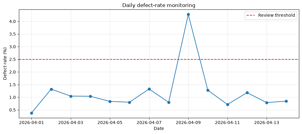
Reading the results

An increase in defect rates and a decrease in the number of reported lines are different anomalies. The former leads to investigations of processes and materials, while the latter leads to checking for input delays and coordination failures. By distinguishing between KPI anomalies and data pipeline anomalies, routing to responsible departments becomes clearer.

No.010: Organizing the Progress of Anomaly Detection Projects

Meaning in Practice

The results of anomaly detection projects are not models, but rather operational outcomes such as loss reduction, avoidance of downtime, and reduction of verification workload. Before starting a PoC, we agree on post-detection actions and methods for measuring effectiveness.

Approach to Analysis and Modeling

The approach is: issue definition→ data audit→ baseline → offline evaluation→ shadow operation→ limited operation→ production and improvement. In addition to model metrics, KPIs include the number of alerts per day, detection lead time, response rate, and avoidance losses.

Check with Python

project_plan = pd.DataFrame([
    [1, "Problem framing", "Target loss and action defined", "Plant manager"],
    [2, "Data audit", "Keys, gaps, labels reviewed", "Data/OT owner"],
    [3, "Baseline", "Rules and simple score compared", "Analytics"],
    [4, "Offline evaluation", "Recall, false alerts, lead time", "Analytics + maintenance"],
    [5, "Shadow operation", "Alerts reviewed without control", "Operators"],
    [6, "Limited rollout", "SOP and escalation validated", "Operations"],
    [7, "Production", "Value and drift monitored", "Cross-functional owner"],
], columns=["step", "phase", "exit_criterion", "primary_owner"])
display(project_plan)

expected = pd.Series({
    "avoided_failures_per_year": 3,
    "loss_per_failure_mjpy": 8.0,
    "annual_operation_cost_mjpy": 6.0,
})
expected["expected_net_value_mjpy"] = (
    expected["avoided_failures_per_year"] * expected["loss_per_failure_mjpy"]
    - expected["annual_operation_cost_mjpy"]
)
display(expected.to_frame("assumption"))

	step	phase	exit_criterion	primary_owner
0	1	Problem framing	Target loss and action defined	Plant manager
1	2	Data audit	Keys, gaps, labels reviewed	Data/OT owner
2	3	Baseline	Rules and simple score compared	Analytics
3	4	Offline evaluation	Recall, false alerts, lead time	Analytics + maintenance
4	5	Shadow operation	Alerts reviewed without control	Operators
5	6	Limited rollout	SOP and escalation validated	Operations
6	7	Production	Value and drift monitored	Cross-functional owner

	assumption
avoided_failures_per_year	3.0
loss_per_failure_mjpy	8.0
annual_operation_cost_mjpy	6.0
expected_net_value_mjpy	18.0

Reading the results

In hypothetical estimates, the annual net effect is 18 million yen, but the number of avoidance cases and loss amounts are uncertain. PoC records not only technical accuracy but also the time from alert to inspection, actual avoided losses, and operational workload, updating investment decisions.

Practical Implications Seen Through Target Exercise

1. Distinguishing the definition of an anomaly: Data quality, statistical anomalies, operational anomalies, and equipment status cannot be condensed into a single flag.
2. Leaving context and time: Without variety, shift, arrangement, and continuity, it is impossible to explain the anomalies that are critical to the site.
3. Decide on actions before methods: Define the confirmer, deadline, inspection details, and escalation at the time of detection.
4. Use simple criteria as a baseline: Advanced models are evaluated by whether they can improve losses and man-hours compared to current rules.
5. Capitalize review results: Structure on-site comments for alerts and use them as future labels and materials for improvement.

What is necessary for practical implementation

• Target losses and KPIs: missed losses, false alarm man-hours, lead time, response rate
• Data Infrastructure: Unified IDs for equipment, lots, and time, time synchronization, and loss monitoring
• Operational design: alert levels, SOPs, demarcation of responsibility, suspension authority, audit trail
• Evaluation Design: Shadow operations, on-site reviews, and verification across periods and seasons
• Continuous improvement: monitoring distribution changes through process changes, sensor replacements, and new product varieties
• Governance: Prioritizing safety and quality standards over models, clearly specifying the scope of human final judgment.

Conclusion

The starting point for anomaly detection is not algorithms, but “what happens when it happens, who does what.” By distinguishing between outliers, outliers, and abnormal states, statistical and operational anomalies, and point, context, and group anomalies, data processing and on-site response can be correctly designed. From the next chapter onward, we will progressively move on to preprocessing, statistical methods, time series, multivariates, and machine learning.

Consultations for Corporations

At Suri Kobo, we support manufacturing anomaly detection PoC, data diagnostics, model development, on-site operations design, and corporate training. You can consult from stages such as “We have data but can’t narrow down themes,” “Alerts aren’t used often,” or “We want to connect PoC to production operations.”

📩 Contact Us: surikobo.co.jp/contact
Please feel free to consult us first.