Capturing the “Usual” Difference in Equipment Sensors: 10 Anomaly Detection Exercises Using Deep Learning (No.071–No.080)

In this article, we use a fictional motor assembly line as the subject and consistently examine anomaly detection using Autoencoder reconstruction errors, covering concepts, implementation, thresholds, time series, and operational decisions. The goal is to provide materials for maintenance personnel to decide which equipment to check and when, especially in manufacturing sites where correct labels are scarce.

[!NOTE] This material is a notebook previously used by Surikoubo (or personally by the representative, Kazuyama), and has been reconstructed, edited, and published with the company’s permission. All data listed is fictional and has no relation whatsoever to real companies, factories, or figures.

Introduction: Practical Challenges in Manufacturing Covered in This Article

The vibration, temperature, current, sound pressure, and rotational speed of the motor are interrelated. In univariate upper limit monitoring, even if each value falls within the specification, signs such as “high temperature relative to load” or “abnormal combinations of rotational speed and vibration” are missed. In this article, we learn the relationship between normal driving and rank observations that are difficult to restore as candidate inspection candidates.

Common situations on site

• There are few fault labels, but there are a large number of logs during normal operation
• The normal range varies depending on the variety, load, and time of day.
• Frequent false reports cause alerts to be ignored.
• Even high-precision models cannot be valued if they cannot be connected to the maintenance flow.

Why is this issue so difficult to judge?

Abnormalities are rare and their types change. Therefore, it is difficult to learn all patterns from past failures alone. Also, a large reconstruction error does not prove failure, but merely indicates a deviation from the learned normal pattern. Thresholds must be determined not only based on statistical evidence but also on missed losses, inspection capability, and process downtime risks.

Overview of Exercise covered this time

In No.071–075, we construct an Autoencoder for tabular sensors and handle reconstruction errors and thresholds. In No.076–078, we consider extensions to time series, LSTM, and images; in No.079, we organize the criteria for overfitting; and in No.080, we organize the criteria for practical hiring.

Preparing the Python environment

It does not depend on external data. For reproducibility, the random number seed is fixed, and the graph is drawn using matplotlib. Here, to avoid requiring additional deep learning foundations, we implement the same “reconstruct input” training as Autoencoder in multilayer neural networks. In actual projects, it is possible to replace it with PyTorch or TensorFlow.

import sys
import warnings
import numpy as np
import pandas as pd
import matplotlib
import matplotlib.pyplot as plt
from sklearn.neural_network import MLPRegressor
from sklearn.preprocessing import StandardScaler
from sklearn.metrics import confusion_matrix

warnings.filterwarnings("ignore", category=UserWarning)
SEED = 42
rng = np.random.default_rng(SEED)
pd.set_option("display.max_columns", 20)
print(f"Python: {sys.version.split()[0]}")
print(f"numpy: {np.__version__}, pandas: {pd.__version__}, matplotlib: {matplotlib.__version__}")

Python: 3.13.1
numpy: 2.5.1, pandas: 3.0.3, matplotlib: 3.11.0

Creation of Fictional Data

Generate 2,400 motor operation logs at 5-minute intervals. The first 1,600 records are used as “normal history” for training, while the second 800 records are mixed with normal data and three types of fictional abnormalities (bearing degradation, cooling failure, load fluctuations). In practice, it is important to cross-check with equipment history to ensure there are no stoppages, replacements, or known abnormalities during the training period.

n = 2400
t = np.arange(n)
load = np.clip(65 + 12*np.sin(2*np.pi*t/288) + rng.normal(0, 5, n), 35, 95)
rpm = 1450 + 4.2*load + rng.normal(0, 18, n)
current = 8 + 0.16*load + rng.normal(0, 0.45, n)
temperature = 31 + 0.34*load + 0.7*np.sin(2*np.pi*t/576) + rng.normal(0, 0.8, n)
vibration = 0.55 + 0.010*load + rng.normal(0, 0.07, n)
sound = 61 + 0.055*rpm/10 + 1.8*vibration + rng.normal(0, 0.7, n)

labels = np.zeros(n, dtype=int)
anomaly_type = np.full(n, "normal", dtype=object)
idx_bearing = np.arange(1780, 1810)
idx_cooling = np.arange(2040, 2070)
idx_load = np.arange(2260, 2285)
vibration[idx_bearing] += np.linspace(0.35, 1.15, len(idx_bearing)); sound[idx_bearing] += 3.8
temperature[idx_cooling] += np.linspace(4, 10, len(idx_cooling)); current[idx_cooling] += 1.2
rpm[idx_load] += rng.choice([-1, 1], len(idx_load))*rng.uniform(90, 170, len(idx_load)); current[idx_load] += 2.0
for idx, name in [(idx_bearing,"bearing"),(idx_cooling,"cooling"),(idx_load,"load_shift")]:
    labels[idx] = 1; anomaly_type[idx] = name

features = ["load_pct","rpm","current_a","temperature_c","vibration_mm_s","sound_db"]
df = pd.DataFrame({"timestamp": pd.date_range("2026-01-01", periods=n, freq="5min"),
                   "load_pct":load,"rpm":rpm,"current_a":current,"temperature_c":temperature,
                   "vibration_mm_s":vibration,"sound_db":sound,
                   "is_anomaly":labels,"anomaly_type":anomaly_type})
print(df.shape)
df.head().round(2)

(2400, 9)

	timestamp	load_pct	rpm	current_a	temperature_c	vibration_mm_s	sound_db	is_anomaly	anomaly_type
0	2026-01-01 00:00:00	66.52	1721.37	18.66	54.30	1.21	72.43	0	normal
1	2026-01-01 00:05:00	60.06	1719.90	17.85	52.02	1.20	72.66	0	normal
2	2026-01-01 00:10:00	69.28	1746.02	19.08	55.00	1.30	72.08	0	normal
3	2026-01-01 00:15:00	70.49	1733.49	19.72	55.05	1.26	71.84	0	normal
4	2026-01-01 00:20:00	56.29	1670.83	16.80	49.75	1.18	72.44	0	normal

No.071: Understanding the Concept of Anomaly Detection with Autoencoder

Meaning in Practice

It learns sensor relationships during normal conditions and can select drivers that deviate from those relationships as candidates for inspection. Instead of models that name faults, it screens for “driving different from usual” that includes unknown signs.

Approach to Analysis and Modeling

Autoencoder compresses input $\mathbf{x}$ into a low-dimensional representation $\mathbf{z}=f_\theta(\mathbf{x})$ and restores it to $\hat{\mathbf{x}}=g_\phi(\mathbf{z})$. Mean squared error with normal data

$L(\theta,\phi)=\frac{1}{n}\sum_{i=1}^{n}\lVert\mathbf{x}_i-\hat{\mathbf{x}}_i\rVert_2^2$

If you reduce it, it is expected that normal patterns are easier to restore, while unlearned patterns are harder to restore. However, if the model size is too large, it can be restored to abnormal levels effectively, so compression and regularization are necessary.

Check with Python

First, standardize and define a network that compresses the input 6D into a 3D bottleneck.

train_end = 1600
scaler = StandardScaler()
X_train = scaler.fit_transform(df.loc[:train_end-1, features])
X_all = scaler.transform(df[features])
ae = MLPRegressor(hidden_layer_sizes=(8, 3, 8), activation="tanh", solver="adam",
                  alpha=0.001, max_iter=500, random_state=SEED, early_stopping=True,
                  validation_fraction=0.15, n_iter_no_change=25)
print(ae)

MLPRegressor(activation='tanh', alpha=0.001, early_stopping=True,
             hidden_layer_sizes=(8, 3, 8), max_iter=500, n_iter_no_change=25,
             random_state=42, validation_fraction=0.15)

Reading the results

By setting bottlenecks, you teach them not just copies of values, but the main correlation structures. Standardization prevents only variables with large digits, like rpm, from controlling losses.

No.072: Implementing a Simple Autoencoder

Meaning in Practice

In PoC, before complex models, it is verified whether a small network can reproduce normal operation. Training time, reproducibility, and relearning procedures are operational requirements just like accuracy.

Approach to Analysis and Modeling

Only the normal period is given to both the input and the objective variable. When the evaluation target is mixed into learning, data leakage occurs where abnormalities are remembered as normal.

Check with Python

ae.fit(X_train, X_train)
train_recon = ae.predict(X_train)
print(f"Number of Repetitions: {ae.n_iter_}")
print(f"Mean reconstruction error of normal training data: {np.mean((X_train-train_recon)**2):.4f}")
print(f"Final Studyloss: {ae.loss_:.4f}")

Number of study repetitions: 500
Mean reconstruction error of normal training data: 0.0455
Final learning loss: 0.0228

Reading the results

A small mean error indicates the reproducibility of normal history, but it does not guarantee anomaly detection performance alone. Next, the error of the observation unit is calculated, and the normal period and evaluation period are separated and compared.

No.073: Calculating Reconstruction Error

Meaning in Practice

By assigning an abnormality score to each equipment log, you can establish the priority of patrol inspections. Furthermore, variable-specific errors are not for cause investigation but are candidates for the “sensor to check first.”

Approach to Analysis and Modeling

Let the score for observation $i$ be $e_i=\frac{1}{p}\sum_{j=1}^{p}(x_{ij}-\hat{x}_{ij})^2$. Because calculations are done in a standardized space, sensors from different units can be compared.

Check with Python

X_recon = ae.predict(X_all)
sq_error = (X_all-X_recon)**2
df["reconstruction_error"] = sq_error.mean(axis=1)
for j, col in enumerate(features):
    df[f"err_{col}"] = sq_error[:, j]
top = df.loc[train_end:].nlargest(8, "reconstruction_error")
top[["timestamp","anomaly_type","reconstruction_error"] + [f"err_{c}" for c in features]].round(3)

	timestamp	anomaly_type	reconstruction_error	err_load_pct	err_rpm	err_current_a	err_temperature_c	err_vibration_mm_s	err_sound_db
1809	2026-01-07 06:45:00	bearing	14.955	1.540	1.648	2.499	1.800	62.548	19.692
1808	2026-01-07 06:40:00	bearing	14.435	2.922	1.237	2.817	4.001	61.959	13.675
1804	2026-01-07 06:20:00	bearing	11.719	2.548	0.798	2.310	1.023	44.297	19.336
1801	2026-01-07 06:05:00	bearing	10.634	1.556	3.690	2.012	1.476	41.910	13.158
1805	2026-01-07 06:25:00	bearing	9.941	4.848	4.123	6.508	1.469	32.806	9.892
1807	2026-01-07 06:35:00	bearing	9.926	2.612	1.218	3.052	2.127	41.054	9.493
1802	2026-01-07 06:10:00	bearing	9.426	2.579	1.490	2.222	1.616	32.748	15.901
1803	2026-01-07 06:15:00	bearing	9.398	3.134	0.549	3.252	2.999	33.328	13.125

Reading the results

In higher-level logs, errors such as vibration and sound pressure increase if bearing abnormalities, and temperature and other errors increase if cooling abnormalities occur. However, since the errors of each variable are affected by correlation, determining the cause of failure requires physical inspection and maintenance records.

No.074: Visualizing the Distribution of Reconstruction Error

Meaning in Practice

By looking not only at the average but also at the tail end of the distribution, you can gauge how likely false alarms are and whether abnormal groups separate from normal groups.

Approach to Analysis and Modeling

Since errors tend to be long distributions to the right, check the histogram using the logarithmic line. Labels are used solely for post-evaluation, not for model training.

Check with Python

normal_eval = df.loc[(df.index>=train_end) & (df.is_anomaly==0), "reconstruction_error"]
anomaly_eval = df.loc[(df.index>=train_end) & (df.is_anomaly==1), "reconstruction_error"]
plt.figure(figsize=(9,4.5))
plt.hist(normal_eval, bins=45, alpha=.7, label="normal", color="#4C78A8")
plt.hist(anomaly_eval, bins=30, alpha=.7, label="injected anomaly", color="#E45756")
plt.yscale("log")
plt.title("Distribution of autoencoder reconstruction error")
plt.xlabel("Mean squared reconstruction error (standardized scale)")
plt.ylabel("Count (log scale)")
plt.grid(True, alpha=.3); plt.legend(); plt.tight_layout(); plt.show()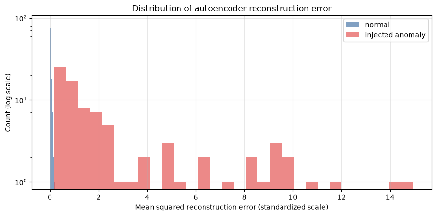

Reading the results

If the error of the abnormal group shifts to the right, it may be useful for selecting inspection candidates. Since there is overlap, it does not automatically stop based solely on scores; instead, it operates gradually based on the number of consecutive alarms or combinations with other alarms.

No.075: Setting a Threshold for Reconstruction Error

Meaning in Practice

Thresholds represent the number of inspections and the conditions for missing cases. Designs exceeding the number of cases the site can check per day will not continue.

Approach to Analysis and Modeling

Let the 99th percentile of normal learning error be the provisional threshold $\tau=Q_{0.99}(e)$. This does not mean a 99% failure rate. This is an operational standard that exceeds the normal history by about 1%.

Check with Python

threshold = np.quantile(df.loc[:train_end-1,"reconstruction_error"], .99)
eval_df = df.loc[train_end:].copy()
eval_df["detected"] = (eval_df["reconstruction_error"] > threshold).astype(int)
tn, fp, fn, tp = confusion_matrix(eval_df.is_anomaly, eval_df.detected).ravel()
metrics = pd.Series({"threshold":threshold,"alerts":int(eval_df.detected.sum()),
                     "precision":tp/(tp+fp),"recall":tp/(tp+fn),
                     "false_positive_rate":fp/(fp+tn)})
metrics.round(3)

threshold               0.189
alerts                 91.000
precision               0.912
recall                  0.976
false_positive_rate     0.011
dtype: float64

Reading the results

Recall is the percentage of embedded anomalies picked up, while Precision is the proportion of anomalies during alerts. In practice, since fault labels are incomplete, logs that appear to be false positives may actually be unrecorded. Assessment results are accumulated through conservation reviews and thresholds are updated.

No.076: Entering Time Series Data into Autoencoder

Meaning in Practice

Even if a single point in time is normal, rapid rises, cycle disruptions, and gentle drifts are abnormal in terms of time sequence. By using the last 12 points (1 hour) as one input, you can handle the shape of change.

Approach to Analysis and Modeling

The window length is determined based on the time scale of the phenomenon to be detected and the notification delay. If you stack windows, the samples are no longer independent, so evaluation is done in chronological order rather than random division.

Check with Python

seq_features = ["current_a","temperature_c","vibration_mm_s"]
seq_scaler = StandardScaler().fit(df.loc[:train_end-1,seq_features])
Z = seq_scaler.transform(df[seq_features])
window = 12
X_seq = np.array([Z[i-window+1:i+1].ravel() for i in range(window-1,n)])
end_index = np.arange(window-1,n)
train_mask = end_index < train_end
seq_ae = MLPRegressor(hidden_layer_sizes=(12,4,12), activation="tanh", max_iter=400,
                      alpha=.002, random_state=SEED, early_stopping=True, n_iter_no_change=20)
seq_ae.fit(X_seq[train_mask], X_seq[train_mask])
seq_error = np.mean((X_seq-seq_ae.predict(X_seq))**2, axis=1)
plt.figure(figsize=(10,4))
plt.plot(df.timestamp.iloc[end_index], seq_error, lw=.8, color="#4C78A8")
plt.axhline(np.quantile(seq_error[train_mask],.99), color="#E45756", ls="--", label="99% threshold")
plt.title("Sequence autoencoder error over time")
plt.xlabel("Timestamp"); plt.ylabel("Window reconstruction error")
plt.grid(True, alpha=.3); plt.legend(); plt.tight_layout(); plt.show()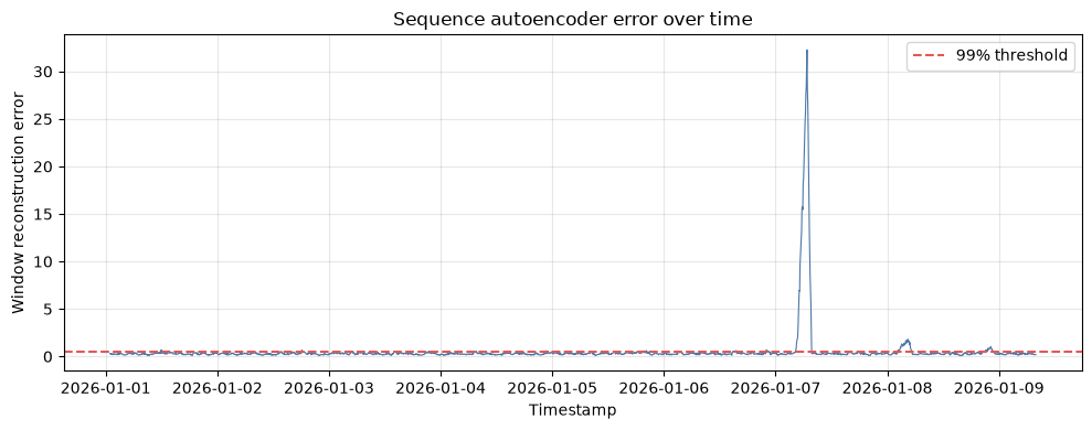

Reading the results

Window-type scores remain high for a while after the anomaly begins. Therefore, instead of the number of alerts, it is necessary to group consecutive excess events as a single event. If the window length is 12, the maximum history of about 55 minutes is included in the interpretation of notification times.

No.077: Understanding the Concept of LSTM Autoencoder

Meaning in Practice

LSTM Autoencoder is a candidate for longer history or if driving order is meaningful. This applies to phenomena like the heating and cooling processes, where the meaning of the same set of values changes depending on the order.

Approach to Analysis and Modeling

LSTM retains historical information through a gate mechanism and restores the series by encoding it into latent representations. On the other hand, learning, reasoning, and monitoring become heavier. Here, as a diagnostic before increasing implementations, check whether the current model’s error changes in the window with disrupted chronological order.

Check with Python

sample_windows = X_seq[~train_mask][:120].reshape(-1,window,len(seq_features))
reversed_windows = sample_windows[:,::-1,:].reshape(-1,window*len(seq_features))
ordered_windows = sample_windows.reshape(-1,window*len(seq_features))
comparison = pd.DataFrame({
    "input":["ordered sequence","reversed sequence"],
    "mean_error":[np.mean((ordered_windows-seq_ae.predict(ordered_windows))**2),
                  np.mean((reversed_windows-seq_ae.predict(reversed_windows))**2)]})
comparison.round(4)

	input	mean_error
0	ordered sequence	0.3374
1	reversed sequence	0.3395

Reading the results

If the error changes due to order reversal, the sequence sequence serves as identification material. However, this fully coupled model does not explicitly represent the temporal structure. If long-term dependence is expected to improve and there is sufficient normal series and computational infrastructure, LSTM can be considered as a comparison candidate.

No.078: Understanding the Concept of Abnormality Detection in Image Data

Meaning in Practice

Visual inspections may not cover all types of scratches, chips, or stains. If you can indicate areas where it is difficult to restore local patterns in normal images, you can narrow down the areas inspected by inspectors.

Approach to Analysis and Modeling

In practice, convolutional Autoencoders and pre-learning features are used. What matters is fixing and aligning imaging conditions, and properly defining product models accordingly. Here, we will examine only how to read the reconstruction error map based on the difference between the hypothetical surface image and the smoothed restoration.

Check with Python

size=48
yy,xx=np.mgrid[:size,:size]
normal_img=.55+.08*np.sin(xx/3)+.06*np.cos(yy/5)+rng.normal(0,.018,(size,size))
defect_img=normal_img.copy(); defect_img[19:24,12:37] -= .30
def smooth(a):
    p=np.pad(a,1,mode="reflect")
    return sum(p[i:i+size,j:j+size] for i in range(3) for j in range(3))/9
reconstructed=smooth(defect_img)
error_map=(defect_img-reconstructed)**2
fig,ax=plt.subplots(1,3,figsize=(10,3.2))
for a,img,title in zip(ax,[defect_img,reconstructed,error_map],["Inspection image","Reconstructed","Squared error map"]):
    im=a.imshow(img,cmap="gray" if title!="Squared error map" else "magma")
    a.set_title(title); a.set_xlabel("X pixel"); a.set_ylabel("Y pixel"); a.grid(False)
fig.suptitle("Conceptual image anomaly localization")
plt.tight_layout(); plt.show()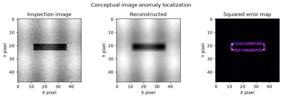

Reading the results

Bright areas on the error map are candidates for confirmation. However, lighting unevenness and misalignment also strongly affect the condition. In image model implementation, standardization of lighting, distance, exposure, background, and model switching determines success or failure before algorithms.

No.079: Checking Overlearning in Deep Learning Models

Meaning in Practice

Models that only reconstruct training data well may falsely report new normal lots. You need to check for generalization across equipment, seasons, and varieties.

Approach to Analysis and Modeling

The normal history is divided by time into 80% for training and 20% for validation, and the error is compared for each iteration. If the learning error continues to decrease while the validation error increases, it is a sign of overlearning. Early termination, model reduction, regularization, and diversification of training periods are all countermeasures.

Check with Python

split=int(len(X_train)*.8); Xa,Xv=X_train[:split],X_train[split:]
monitor=MLPRegressor(hidden_layer_sizes=(20,8,20), activation="tanh", solver="adam",
                     alpha=1e-5, max_iter=1, warm_start=True, random_state=SEED)
train_curve=[]; valid_curve=[]
for epoch in range(80):
    monitor.fit(Xa,Xa)
    train_curve.append(np.mean((Xa-monitor.predict(Xa))**2))
    valid_curve.append(np.mean((Xv-monitor.predict(Xv))**2))
best_epoch=int(np.argmin(valid_curve))+1
plt.figure(figsize=(8,4))
plt.plot(train_curve,label="train"); plt.plot(valid_curve,label="time-based validation")
plt.axvline(best_epoch-1,color="#E45756",ls="--",label=f"best epoch={best_epoch}")
plt.title("Learning curves for overfitting monitoring")
plt.xlabel("Epoch"); plt.ylabel("Reconstruction MSE")
plt.grid(True,alpha=.3); plt.legend(); plt.tight_layout(); plt.show()
print(f"The smallest verification errorepoch: {best_epoch}, minimum value: {min(valid_curve):.4f}")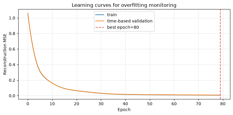

Minimum verification error epoch: 80, minimum value: 0.0083

Reading the results

The number of iterations to be adopted is not the minimum learning error but the minimum time-order validation error as a candidate point. Furthermore, separate days and lots are left as complete holdouts, and the same monitoring continues even after data updates.

No.080: Organizing Criteria for Using Deep Learning in Practice

Meaning in Practice

Deep learning is not the goal. Compared to existing management charts and rules, it is adopted when it helps reduce downtime losses, shorten inspection time, and prevent quality leakage.

Approach to Analysis and Modeling

We create a simplified decision table that scores data volume, nonlinearity, explainability, maintainability, and inference constraints. This is not an automated pass/fail judgment, but a checklist to align key issues in manufacturing, maintenance, quality, and IT.

Check with Python

criteria=pd.DataFrame({
 "judgment item":["Volume and Coverage of Normal Data","The Need for Nonlinear, Image, and Long-Term Series","Verifiability of False Reports and Missed Accounts",
          "Auxiliary design for explanation and cause investigation","Relearning, Version Management, and Monitoring System","Time and Computational Constraints in Edge Inference"],
 "Current Status Score(1-5)":[4,4,3,2,2,4],
 "GoGuidelines":["Including multiple conditions and seasons","Examining the difference from the simple method","Ability to record conservation results",
           "Variable-based errors, etc. included","There is a responsible person and renewal procedures.","Stable operation within the required time"]})
criteria["Response Required"] = criteria["Current Status Score(1-5)"] < 3
display(criteria)
print("provisional judgment:", "With a limited line,PoC" if criteria["Current Status Score(1-5)"].mean()>=3 else "Establishing Data and Operational Infrastructure First")

	judgment item	Current Status Score(1-5)	GoGuidelines	Response Required
0	Volume and Coverage of Normal Data	4	Including multiple conditions and seasons	False
1	The Need for Nonlinear, Image, and Long-Term Series	4	Examining the difference from the simple method	False
2	Verifiability of False Reports and Missed Accounts	3	Ability to record conservation results	False
3	Auxiliary design for explanation and cause investigation	2	Variable-based errors, etc. included	True
4	Relearning, Version Management, and Monitoring System	2	There is a responsible person and renewal procedures.	True
5	Time and Computational Constraints in Edge Inference	4	Stable operation within the required time	False

Preliminary judgment: PoC on limited lines

Reading the results

In this example, the data and computational constraints are relatively good, but since the explanation support and model update system are weak, it is more appropriate to use a limited line of PoC rather than a company-wide rollout. Compare baselines, Autoencoder, and operational costs over the same period, and evaluate effectiveness in terms of value and man-hours.

Practical Implications Seen Through Target Exercise

1. Reconstruction error is not the probability of failure, but the degree of deviation from the normal model.
2. Thresholds are determined not only by statistics but also by inspection capability and loss structure.
3. Single-point, time-series, and image definitions and data quality management differ.
4. Before improving performance, we design pollution prevention during the training period, event aggregation, and conservation result recording.
5. The model is not just about issuing alerts; it is a business system that includes judgment, inspection, and feedback.

What is necessary for practical implementation

• Agree on the target equipment, detection lead time, allowable number of false alarms, and the losses to be avoided.
• Manage sensor calibration, missing items, time synchronization, equipment status, types, and maintenance history
• Compare with baseline conditions such as control charts or Isolation Forest
• Designing alerts, check-to-confirm, emergency stage notifications, consecutive exceedances, and deterrence times
• Manage models, features, thresholds, training data, and approvers
• Regularly review drift, number of alerts, inspection results, and avoided losses

Conclusion

In No.071–080, we checked everything from normal pattern learning using Autoencoder to reconstruction errors, thresholds, extensions to time series, LSTM, and images, over-fitting, and adoption decisions. The value of deep learning lies in capturing complex relationships, but the outcome is determined not by the model alone, but by data quality and connection to maintenance operations. First, it is practical to measure differences from the baseline and inspection load within a limited range, then expand from the range where the effect can be reproduced.

Consultations for Corporations

At Mathematical Laboratory, we support from problem organization to problem organization, from anomaly detection PoC in manufacturing industries, evaluation of sensor and image data, threshold and alert operation design, to embedding into existing systems.

📩 Contact Us: surikobo.co.jp/contact Please feel free to consult us first.