
100 Exercises / anomaly detection / Abnormality detection: 100 Exercises
Introduction to Sensor Data Anomaly Detection in Manufacturing | Practical Changes in Sudden Changes, Sticking, and Relationship Breakdown Using Python
Turning Sensor Data Anomalies into ‘Stopping Decisions’: 10 Key Points in Facility Monitoring Practice
This course covers methods for distinguishing between Sensor-Specific Anomalies and Abnormal equipment condition by focusing on temperature, vibration, pressure, and current of manufacturing equipment, and narrowing down the equipment, timing, and possible causes that maintenance personnel should check. The target is the No.041〜No.050(Chapter5Chapter: Sensor Data Anomaly Detection) with 100 Exercises detected for abnormalities.
Instead of judging based solely on a single threshold, we gradually combine sudden changes, adhesions, physical limits, relationships between sensors, and equipment-specific aggregations. It uses fictitious data and does not rely on external data.
[!NOTE] This material is a notebook previously used by Surikoubo (or personally by the representative, Kazuyama), and has been reconstructed, edited, and published with the company’s permission.
All data listed is fictional and has no relation whatsoever to real companies, factories, or figures.
Introduction: Practical Challenges in Manufacturing Covered in This Article
The purpose of equipment monitoring is not to display a large number of anomalous points. The goal is to detect signs that lead to quality defects or sudden stoppages early, supporting Continuous operation, on-site inspection, planned maintenance, emergency shutdown decision-making.
This time, we will assume a site where three identical processing machines are equipped with multiple sensors. Monitors need to quickly distinguish not only from “high values” but also from instrument failures, load fluctuations, or equipment deterioration.
Common situations on site
- Sampling periods, units, and missing data expressions differ for each sensor
- Normal changes caused by starting, stopping, or switching varieties will be alerted
- Communication outages and sensor failures are recorded as “0”
- Even within the normal range alone, the relationship between temperature and current is disrupted
- There are many devices, making it difficult for people to keep viewing individual graphs.
Why is this issue so difficult to judge?
Sensor data is a time series with autocorrelation, and the normal range varies depending on equipment, operating conditions, and aging conditions. Furthermore, statistical anomalies do not coincide with operational risks. Therefore, detection rules must incorporate “physical meaning,” “duration,” “consistency of multiple signals,” and “costs in case of false positives versus missed signals.”
Overview of Exercise covered this time
| No. | Theme | Questions to answer on site |
|---|---|---|
| 041 | Features of Sensor Data | What to check before monitoring |
| 042 | Multiple sensor time series | How to shape it for easy analysis |
| 043 | Distribution by Sensor | How does the usual range and hem width differ? |
| 044 | Rapid Rise and Fall | How to pick up on momentary changes |
| 045 | Zero sticking | How to pick up on continuous zeros that seem to be communication disconnections or failures |
| 046 | Exceeding the upper and lower limits | How to Immediately Determine Violations of Management Standards |
| 047 | Inter-sensor correlation | How to understand normal linkage |
| 048 | relationship breakdown | How to pick up anomalies that can’t be seen with univariate methods |
| 049 | Comparison by Equipment | Which equipment should you check first? |
| 050 | Interpretation from the Field Perspective | How to Turn Detection into Conservation Action |
Detection is not a linear process; rather, judgment materials are stacked in Data Quality → Univariate Rules → Multivariate Consistency → Priority by Equipment → On-site Inspection order.
Preparing the Python environment
Data is created and aggregated in numpy and pandas, visualized in matplotlib. Fixed random number seeds to ensure reproducibility. The graphs are displayed in English to avoid environment-dependent garbling, and reading is explained in detail in the main text.
import sys
import numpy as np
import pandas as pd
import matplotlib
import matplotlib.pyplot as plt
from IPython.display import display

SEED = 42
rng = np.random.default_rng(SEED)
pd.set_option("display.max_columns", 20)
print(f"Python {sys.version.split()[0]} / pandas {pd.__version__} / matplotlib {matplotlib.__version__}")
Python 3.13.1 / pandas 3.0.3 / matplotlib 3.11.0Creation of Fictional Data
Observe equipment A through C for 40 hours at 10-minute intervals. When the current (load) rises, temperature and vibration rise, and the pressure is generated so that it gently works in tandem. On top of that, we embed the vibration spike of equipment B, the zero pressure attachment of equipment C, the temperature rise of equipment A, and the relationship of equipment B where the vibration is only higher than the current. injected_event is for checking answers in teaching materials and usually does not exist in practice.
timestamps = pd.date_range("2026-06-01 08:00", periods=240, freq="10min")
rows = []
offsets = {"EquipmentA": (0.0, 0.00), "EquipmentB": (1.0, 0.08), "EquipmentC": (-0.7, -0.05)}
for machine, (temp_offset, vib_offset) in offsets.items():
    phase = {"EquipmentA": 0.0, "EquipmentB": 0.8, "EquipmentC": 1.6}[machine]
    t = np.arange(len(timestamps))
    load = 64 + 8*np.sin(2*np.pi*t/72 + phase) + rng.normal(0, 2.0, len(t))
    temperature = 38 + temp_offset + 0.36*load + rng.normal(0, 0.8, len(t))
    vibration = 0.75 + vib_offset + 0.018*load + rng.normal(0, 0.07, len(t))
    pressure = 4.0 + 0.020*load + rng.normal(0, 0.08, len(t))
    for i, ts in enumerate(timestamps):
        rows.append([ts, machine, temperature[i], vibration[i], pressure[i], load[i], "normal"])

df = pd.DataFrame(rows, columns=["timestamp", "machine", "temperature_c", "vibration_mm_s", "pressure_mpa", "current_a", "injected_event"])

def inject(machine, start, end, column, operation, label):
    mask = (df["machine"] == machine) & df.groupby("machine").cumcount().between(start, end)
    df.loc[mask, column] = operation(df.loc[mask, column].to_numpy())
    df.loc[mask, "injected_event"] = label

inject("EquipmentB", 75, 75, "vibration_mm_s", lambda x: x + 2.1, "vibration_spike")
inject("EquipmentC", 120, 128, "pressure_mpa", lambda x: np.zeros_like(x), "pressure_zero_stuck")
inject("EquipmentA", 170, 180, "temperature_c", lambda x: x + np.linspace(8, 13, len(x)), "temperature_high")
inject("EquipmentB", 195, 207, "vibration_mm_s", lambda x: x + 0.75, "relation_break")
df = df.sort_values(["machine", "timestamp"]).reset_index(drop=True)

print(f"Number of lines: {len(df):,} / Number of facilities: {df.machine.nunique()} / Period: {df.timestamp.min()} 〜 {df.timestamp.max()}")
display(df.head())
Number of lines: 720 / Number of facilities: 3 / Period: 2026-06-01 08:00:00 〜 2026-06-02 23:50:00| timestamp | machine | temperature_c | vibration_mm_s | pressure_mpa | current_a | injected_event | |
|---|---|---|---|---|---|---|---|
| 0 | 2026-06-01 08:00:00 | EquipmentA | 60.557908 | 1.928585 | 5.284494 | 64.609434 | normal |
| 1 | 2026-06-01 08:10:00 | EquipmentA | 60.466810 | 1.977436 | 5.342587 | 62.617278 | normal |
| 2 | 2026-06-01 08:20:00 | EquipmentA | 60.674249 | 1.960428 | 5.155343 | 66.890088 | normal |
| 3 | 2026-06-01 08:30:00 | EquipmentA | 61.288969 | 2.013785 | 5.239303 | 67.951682 | normal |
| 4 | 2026-06-01 08:40:00 | EquipmentA | 62.323670 | 1.877039 | 5.182851 | 62.834091 | normal |
No.041: Organizing the Features of Sensor Data
Meaning in Practice
From column names alone, you cannot know the units, period, missing measurements, physical range, or calibration history. If you do not check the quality of each signal before creating monitoring rules, you may confuse equipment abnormalities with measurement anomalies.
Approach to Analysis and Modeling
Minimum data type, missing rate, unique number, minimum/maximum, and time interval are kept as data profiles. Signals with extremely few unique counts or continuous values are candidates for sensor attachment. In this 10-minute cycle, one difference represents a 10-minute change.
Check with Python
sensor_cols = ["temperature_c", "vibration_mm_s", "pressure_mpa", "current_a"]
profile = pd.DataFrame({
    "dtype": df[sensor_cols].dtypes.astype(str),
    "missing_rate_pct": df[sensor_cols].isna().mean().mul(100),
    "unique_values": df[sensor_cols].nunique(),
    "min": df[sensor_cols].min(),
    "max": df[sensor_cols].max(),
}).round(3)
intervals = df.groupby("machine")["timestamp"].diff().dropna().value_counts()
display(profile)
print("Main observation intervals:", intervals.index[0], "/ Number of Relevant Lines:", intervals.iloc[0])| dtype | missing_rate_pct | unique_values | min | max | |
|---|---|---|---|---|---|
| temperature_c | float64 | 0.0 | 720 | 55.242 | 75.080 |
| vibration_mm_s | float64 | 0.0 | 720 | 1.568 | 4.222 |
| pressure_mpa | float64 | 0.0 | 712 | 0.000 | 5.669 |
| current_a | float64 | 0.0 | 720 | 50.810 | 76.257 |
Main observation interval: 0 days 00:10:00 / Number of relevant lines: 717Reading the results
There are no defects, and the observation intervals are aligned at 10 minutes. On the other hand, the minimum pressure is zero, which is unnatural for normal operation. You need to check not only the maximum value but also the “impossible value” and “continuity.” In practice, you add the unit, tag ID, range, calibration date, and equipment condition to this table.
No.042: Reading Time Series Data from Multiple Sensors
Meaning in Practice
On-site data is often collected vertically by sensor, and during analysis, it is necessary to line up the data side by side at the same time and with the same equipment. Misalignment in the bond causes a nonexistent correlation breakdown.
Approach to Analysis and Modeling
Set the key to timestamp × machine, check for duplicates, and then switch to wide format. If the times do not match exactly, neighborhood coupling or resampling with allowable times is required. Here, the formatted data is first converted to a long format, and the standard form after loading is checked.
Check with Python
long_df = df.melt(
    id_vars=["timestamp", "machine"], value_vars=sensor_cols,
    var_name="sensor", value_name="value"
)
wide_df = long_df.pivot(index=["timestamp", "machine"], columns="sensor", values="value").reset_index()
duplicate_keys = df.duplicated(["timestamp", "machine"]).sum()
print("longform:", long_df.shape, "/ wideform:", wide_df.shape, "/ key duplication:", duplicate_keys)
display(long_df.head(8))
display(wide_df.head(3))
Long format: (2880, 4) / wide format: (720, 6) / Key duplication: 0| timestamp | machine | sensor | value | |
|---|---|---|---|---|
| 0 | 2026-06-01 08:00:00 | EquipmentA | temperature_c | 60.557908 |
| 1 | 2026-06-01 08:10:00 | EquipmentA | temperature_c | 60.466810 |
| 2 | 2026-06-01 08:20:00 | EquipmentA | temperature_c | 60.674249 |
| 3 | 2026-06-01 08:30:00 | EquipmentA | temperature_c | 61.288969 |
| 4 | 2026-06-01 08:40:00 | EquipmentA | temperature_c | 62.323670 |
| 5 | 2026-06-01 08:50:00 | EquipmentA | temperature_c | 60.289633 |
| 6 | 2026-06-01 09:00:00 | EquipmentA | temperature_c | 61.694617 |
| 7 | 2026-06-01 09:10:00 | EquipmentA | temperature_c | 63.933736 |
| sensor | timestamp | machine | current_a | pressure_mpa | temperature_c | vibration_mm_s |
|---|---|---|---|---|---|---|
| 0 | 2026-06-01 08:00:00 | EquipmentA | 64.609434 | 5.284494 | 60.557908 | 1.928585 |
| 1 | 2026-06-01 08:00:00 | EquipmentB | 72.972598 | 5.339398 | 64.212102 | 2.096983 |
| 2 | 2026-06-01 08:00:00 | EquipmentC | 69.809115 | 5.443274 | 62.014050 | 1.925339 |
Reading the results
Four signals × 720 lines are restored to 2,880 lines in long format and 720 lines in wide format, with no key duplication. In practice, we also check the equipment master for correspondence, time zones, and sampling delays here, so that the shaping process can be redone in the same steps every time.
No.043: Checking the distribution by sensor
Meaning in Practice
By looking at the distribution, you can grasp the normal range, left-right distortion, multiple driving modes, and physically unnatural hems. If all equipment is aggregated at once, equipment differences may be mistaken for abnormalities, so summarizing by equipment is also necessary.
Approach to Analysis and Modeling
It uses not only mean and standard deviation but also median and quantiles. Median values and IQR, which are less susceptible to abnormalities, are effective for setting standards. However, since distributions lose temporal order, detection cannot be completed using only the histogram.
Check with Python
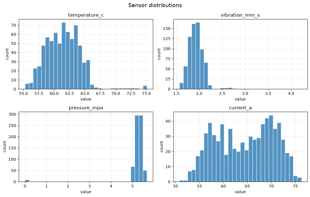
summary = df.groupby("machine")[sensor_cols].agg(["mean", "std", "median", "min", "max"]).round(2)
display(summary)

fig, axes = plt.subplots(2, 2, figsize=(11, 7))
for ax, col in zip(axes.ravel(), sensor_cols):
    ax.hist(df[col], bins=30, color="#2878B5", alpha=0.8, edgecolor="white")
    ax.set_title(col)
    ax.set_xlabel("value")
    ax.set_ylabel("count")
    ax.grid(alpha=0.25)
fig.suptitle("Sensor distributions", fontsize=14)
plt.tight_layout()
plt.show()| temperature_c | vibration_mm_s | pressure_mpa | current_a | |||||||||||||||||
|---|---|---|---|---|---|---|---|---|---|---|---|---|---|---|---|---|---|---|---|---|
| mean | std | median | min | max | mean | std | median | min | max | mean | std | median | min | max | mean | std | median | min | max | |
| machine | ||||||||||||||||||||
| EquipmentA | 61.71 | 3.30 | 61.53 | 55.89 | 75.08 | 1.90 | 0.12 | 1.91 | 1.57 | 2.27 | 5.29 | 0.13 | 5.28 | 4.96 | 5.61 | 64.46 | 5.88 | 65.21 | 52.97 | 76.26 |
| EquipmentB | 62.28 | 2.35 | 62.25 | 55.84 | 67.40 | 2.04 | 0.24 | 2.01 | 1.70 | 4.22 | 5.28 | 0.15 | 5.28 | 4.94 | 5.64 | 64.69 | 6.02 | 65.30 | 53.16 | 74.73 |
| EquipmentC | 60.44 | 2.35 | 60.54 | 55.24 | 65.40 | 1.86 | 0.12 | 1.86 | 1.58 | 2.18 | 5.09 | 1.02 | 5.28 | 0.00 | 5.67 | 64.24 | 6.01 | 64.35 | 50.81 | 76.22 |
Reading the results
Pressure shows an independent peak near zero, while temperature and vibration show an upper bottom. These are the entry points for detailed checks. On the other hand, even if the average vibration of equipment B is relatively high, that alone does not constitute a failure. We make judgments by overlaying equipment-specific criteria with the chronological location of occurrence.
No.044: Detecting Sudden Spikes and Drops in Sensor Values
Meaning in Practice
Momentary shocks, disconnections, and unstable control manifest as sudden changes from the previous value, even if the value itself is within the control range. It is effective for lifting short-term events such as bearing vibration spikes.
Approach to Analysis and Modeling
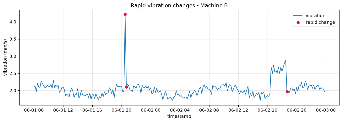
Differences between equipment are defined as , and absolute differences are detected when the operational threshold is exceeded. Since the difference amplifies noise, the threshold is determined based on sensor resolution, period, and the distribution of the normal time difference. This time, we will treat a sudden change where the 10-minute vibration difference exceeds 0.8 mm/s.
Check with Python
df["vibration_diff"] = df.groupby("machine")["vibration_mm_s"].diff()
df["rapid_vibration"] = df["vibration_diff"].abs() > 0.8
rapid = df.loc[df["rapid_vibration"], ["timestamp", "machine", "vibration_mm_s", "vibration_diff", "injected_event"]]
display(rapid.round(3))

b = df[df.machine == "EquipmentB"]
fig, ax = plt.subplots(figsize=(11, 4))
ax.plot(b.timestamp, b.vibration_mm_s, label="vibration", lw=1.3)
hit = b[b.rapid_vibration]
ax.scatter(hit.timestamp, hit.vibration_mm_s, color="crimson", label="rapid change", zorder=3)
ax.set_title("Rapid vibration changes - Machine B")
ax.set_xlabel("timestamp"); ax.set_ylabel("vibration (mm/s)")
ax.grid(alpha=0.3); ax.legend(); plt.tight_layout(); plt.show()
/var/folders/3y/fmw40k0x78xblvb3gkcyvy1h0000gn/T/ipykernel_19414/1863854110.py:4: UserWarning: obj.round has no effect with datetime, timedelta, or period dtypes. Use obj.dt.round(...) instead.
display(rapid.round(3))| timestamp | machine | vibration_mm_s | vibration_diff | injected_event | |
|---|---|---|---|---|---|
| 315 | 2026-06-01 20:30:00 | EquipmentB | 4.222 | 2.258 | vibration_spike |
| 316 | 2026-06-01 20:40:00 | EquipmentB | 2.099 | -2.124 | normal |
| 448 | 2026-06-02 18:40:00 | EquipmentB | 1.969 | -0.912 | normal |
Reading the results
Both spike rise and return are detected. Since two alerts are triggered from a single event, in actual operation, proximity alerts are bundled into one event. It is also important to compare with product switching and startup times to suppress normal sudden changes.
No.045: Detecting zero sticking to sensor values
Meaning in Practice
Continuous zeros may be the result of equipment shutdowns, but they can also occur due to communication outages, disconnections, and sensor failures. If the pressure is zero when other signals indicate operation, the likelihood of a measurement system malfunction increases.
Approach to Analysis and Modeling
Create a zero and count the continuous sections (runs) within the equipment. For floating-point decimals, exact matches are avoided, and a small allowable is allowed. This time, we will focus on three points, meaning sticking for more than 30 minutes of continuous use.
Check with Python
is_zero = df["pressure_mpa"].abs() < 0.01
run_id = (~is_zero).groupby(df["machine"]).cumsum()
df["zero_run_length"] = is_zero.groupby([df["machine"], run_id]).transform("sum")
df["pressure_zero_stuck"] = is_zero & (df["zero_run_length"] >= 3)
stuck_summary = (df[df.pressure_zero_stuck]
    .groupby("machine").agg(start=("timestamp", "min"), end=("timestamp", "max"), points=("timestamp", "size"), mean_current_a=("current_a", "mean")))
display(stuck_summary.round(2))
/var/folders/3y/fmw40k0x78xblvb3gkcyvy1h0000gn/T/ipykernel_19414/85408853.py:7: UserWarning: obj.round has no effect with datetime, timedelta, or period dtypes. Use obj.dt.round(...) instead.
display(stuck_summary.round(2))| start | end | points | mean_current_a | |
|---|---|---|---|---|
| machine | ||||
| EquipmentC | 2026-06-02 04:00:00 | 2026-06-02 05:20:00 | 9 | 63.23 |
Reading the results
Nine points of zero pressure adhesion were detected at Equipment C, and current continued to flow during that time. Therefore, it is reasonable to prioritize checking pressure sensors or communication paths over simple equipment shutdown. If there is a PLC operating flag, this separation becomes even more certain.
No.046: Detecting Sensor Values Exceeding Upper and Lower Limits
Meaning in Practice
Upper and lower limits derived from safety, quality, and equipment specifications are clear operational rules that should take precedence over statistical models. Immediate notification of entry into danger zones, and alert zones by monitoring duration, allowing for phased design.
Approach to Analysis and Modeling
For example, the control range is a temperature of 70°C, vibration of 3.0 mm/s, pressure of 4.7–5.7 MPa, and current of 45–85 A. This is a hypothesis in the teaching materials, and in practice, approval is made by equipment and type based on manufacturer specifications, process capability, quality impact, and measurement errors.
Check with Python
limits = {
    "temperature_c": (None, 70.0),
    "vibration_mm_s": (None, 3.0),
    "pressure_mpa": (4.7, 5.7),
    "current_a": (45.0, 85.0),
}
limit_flags = []
for col, (lower, upper) in limits.items():
    flag = pd.Series(False, index=df.index)
    if lower is not None: flag |= df[col] < lower
    if upper is not None: flag |= df[col] > upper
    name = f"limit_{col}"
    df[name] = flag
    limit_flags.append(name)
df["any_limit_violation"] = df[limit_flags].any(axis=1)
limit_counts = df.groupby("machine")[limit_flags].sum().astype(int)
display(limit_counts)
display(df[df.any_limit_violation][["timestamp", "machine", *sensor_cols, "injected_event"]].head(12).round(2))| limit_temperature_c | limit_vibration_mm_s | limit_pressure_mpa | limit_current_a | |
|---|---|---|---|---|
| machine | ||||
| EquipmentA | 10 | 0 | 0 | 0 |
| EquipmentB | 0 | 1 | 0 | 0 |
| EquipmentC | 0 | 0 | 9 | 0 |
/var/folders/3y/fmw40k0x78xblvb3gkcyvy1h0000gn/T/ipykernel_19414/3734468854.py:18: UserWarning: obj.round has no effect with datetime, timedelta, or period dtypes. Use obj.dt.round(...) instead.
display(df[df.any_limit_violation][["timestamp", "machine", *sensor_cols, "injected_event"]].head(12).round(2))| timestamp | machine | temperature_c | vibration_mm_s | pressure_mpa | current_a | injected_event | |
|---|---|---|---|---|---|---|---|
| 171 | 2026-06-02 12:30:00 | EquipmentA | 70.03 | 2.01 | 5.37 | 70.55 | temperature_high |
| 172 | 2026-06-02 12:40:00 | EquipmentA | 71.02 | 2.09 | 5.33 | 68.23 | temperature_high |
| 173 | 2026-06-02 12:50:00 | EquipmentA | 71.91 | 1.86 | 5.33 | 66.14 | temperature_high |
| 174 | 2026-06-02 13:00:00 | EquipmentA | 71.33 | 1.97 | 5.28 | 65.44 | temperature_high |
| 175 | 2026-06-02 13:10:00 | EquipmentA | 73.04 | 1.99 | 5.44 | 67.73 | temperature_high |
| 176 | 2026-06-02 13:20:00 | EquipmentA | 75.03 | 1.95 | 5.34 | 69.89 | temperature_high |
| 177 | 2026-06-02 13:30:00 | EquipmentA | 74.46 | 1.96 | 5.26 | 66.39 | temperature_high |
| 178 | 2026-06-02 13:40:00 | EquipmentA | 73.40 | 2.01 | 5.34 | 65.15 | temperature_high |
| 179 | 2026-06-02 13:50:00 | EquipmentA | 75.08 | 1.90 | 5.18 | 65.27 | temperature_high |
| 180 | 2026-06-02 14:00:00 | EquipmentA | 75.05 | 1.83 | 5.36 | 66.61 | temperature_high |
| 315 | 2026-06-01 20:30:00 | EquipmentB | 64.57 | 4.22 | 5.47 | 70.98 | vibration_spike |
| 600 | 2026-06-02 04:00:00 | EquipmentC | 60.63 | 1.80 | 0.00 | 62.05 | pressure_zero_stuck |
Reading the results
The high temperature of equipment A, the vibration limit of equipment B exceeding the lower limit, and the lower pressure limit of equipment C are recorded. However, the handling differs between exceeding one point and overstaying for a long time. At implementation, it will include multiple levels of alertness, abnormality, and danger, hysteresis on the returning side, and continuation points to prevent repeated notifications near boundaries.
No.047: Confirm Correlations Between Sensors
Meaning in Practice
The equipment’s signals are not independent. As the load current increases, heat generation and vibration also increase, resulting in physical interactions. By understanding this normal relationship, we can consider anomalies where “values are within the normal range but combinations are unnatural.”
Approach to Analysis and Modeling
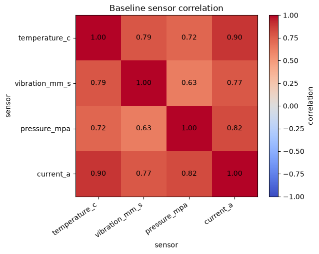
The Pearson correlation coefficient summarizes linear relationships from to . Since we are drawn to anomalies, we first calculate based on baseline data excluding known and obvious control limit violations. Note that correlation is not causal but can change even when driving modes are mixed.
Check with Python
baseline = df[df.injected_event == "normal"]
corr = baseline[sensor_cols].corr()
display(corr.round(2))

fig, ax = plt.subplots(figsize=(6.5, 5.2))
im = ax.imshow(corr, cmap="coolwarm", vmin=-1, vmax=1)
ax.set_xticks(range(len(sensor_cols)), sensor_cols, rotation=35, ha="right")
ax.set_yticks(range(len(sensor_cols)), sensor_cols)
for i in range(len(sensor_cols)):
    for j in range(len(sensor_cols)):
        ax.text(j, i, f"{corr.iloc[i,j]:.2f}", ha="center", va="center")
ax.set_title("Baseline sensor correlation")
ax.set_xlabel("sensor"); ax.set_ylabel("sensor"); ax.grid(False)
fig.colorbar(im, ax=ax, label="correlation")
plt.tight_layout(); plt.show()| temperature_c | vibration_mm_s | pressure_mpa | current_a | |
|---|---|---|---|---|
| temperature_c | 1.00 | 0.79 | 0.72 | 0.90 |
| vibration_mm_s | 0.79 | 1.00 | 0.63 | 0.77 |
| pressure_mpa | 0.72 | 0.63 | 1.00 | 0.82 |
| current_a | 0.90 | 0.77 | 0.82 | 1.00 |
Reading the results
A positive correlation is observed between current and temperature, vibration, and pressure, reflecting common load fluctuations. A high correlation does not necessarily mean you can remove one of them. Since temperature represents heat and vibration represents mechanical condition, it is used for relationship monitoring while retaining its physical role.
No.048: Detecting Relationship Breakdowns Between Sensors
Meaning in Practice
For example, if the current is normal but only vibration increases, the increase in load cannot be explained, and candidates such as imbalance or looseness arise. Signs may be picked up before the simple vibration limit is reached.
Approach to Analysis and Modeling
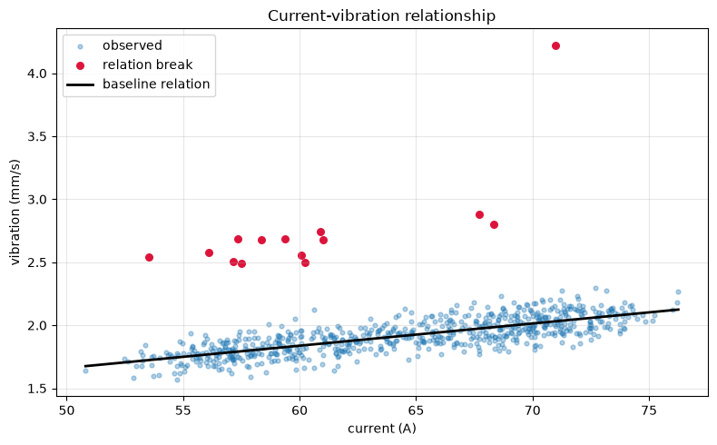
It learns a straight line that explains vibration from current in normal data and calculates the residual . From the median of the normal residual and MAD (Central Absolute Deviation), a robust scale is created, and points where the residual exceeds 4 scales ± the median are considered relationship breakdowns. This is a simple model for explanation; if there are multiple operating modes, a mode-specific model is required.
Check with Python
train = df[df.injected_event == "normal"]
slope, intercept = np.polyfit(train.current_a, train.vibration_mm_s, 1)
df["vibration_expected"] = intercept + slope * df.current_a
df["relation_residual"] = df.vibration_mm_s - df.vibration_expected
train_resid = train.vibration_mm_s - (intercept + slope * train.current_a)
center = train_resid.median()
robust_sigma = 1.4826 * (train_resid - center).abs().median()
df["relation_break_flag"] = (df.relation_residual - center).abs() > 4 * robust_sigma
print(f"anticipatory: vibration = {intercept:.3f} + {slope:.4f} × current")
print(f"Number of Relationship Breakdown Detections: {df.relation_break_flag.sum()} point")

fig, ax = plt.subplots(figsize=(8, 5))
ax.scatter(df.current_a, df.vibration_mm_s, s=12, alpha=0.35, label="observed")
flag = df[df.relation_break_flag]
ax.scatter(flag.current_a, flag.vibration_mm_s, s=30, color="crimson", label="relation break")
x = np.linspace(df.current_a.min(), df.current_a.max(), 100)
ax.plot(x, intercept+slope*x, color="black", lw=2, label="baseline relation")
ax.set_title("Current-vibration relationship")
ax.set_xlabel("current (A)"); ax.set_ylabel("vibration (mm/s)")
ax.grid(alpha=0.3); ax.legend(); plt.tight_layout(); plt.show()
Expectation formula: vibration = 0.780 + 0.0176 × current
Number of relationship breakdown detections: 14 points
Reading the results
A collection of high vibrations that cannot be explained by electric current becomes visible. While sudden change detection is strong against instantaneous spikes, relationship breakdown responds to mild, persistent abnormalities. Since the cause is not definitive, imbalance, wear, and loose fixing are identified by considering rotation speed, processing type, and tool replacement history.
No.049: Comparing abnormal trends by equipment
Meaning in Practice
Conservation resources are limited. Compare not only the total number of alerts but also the type of anomaly, duration, and equipment-specific baselines to prioritize inspections.
Approach to Analysis and Modeling
Detection rules are aggregated by equipment, and even if multiple rules react at the same time, they are grouped into a single “anomaly.” Here, for explanation, we create weighted scores of 2 points for management limit, 1 point for relationship breakdown, 1 point for sudden changes, and 2 points for sticking. Weights should be determined by on-site agreement based on stopping losses and safety impacts.
Check with Python
df["priority_score"] = (
    2*df.any_limit_violation.astype(int)
    + df.relation_break_flag.astype(int)
    + df.rapid_vibration.astype(int)
    + 2*df.pressure_zero_stuck.astype(int)
)
machine_summary = df.groupby("machine").agg(
    limit_points=("any_limit_violation", "sum"),
    rapid_points=("rapid_vibration", "sum"),
    stuck_points=("pressure_zero_stuck", "sum"),
    relation_break_points=("relation_break_flag", "sum"),
    total_priority_score=("priority_score", "sum"),
    max_temperature_c=("temperature_c", "max"),
    max_vibration_mm_s=("vibration_mm_s", "max"),
).sort_values("total_priority_score", ascending=False)
display(machine_summary.round(2))

fig, ax = plt.subplots(figsize=(8, 4.5))
machine_summary[["limit_points", "rapid_points", "stuck_points", "relation_break_points"]].plot.bar(ax=ax)
ax.set_title("Anomaly signals by machine")
ax.set_xlabel("machine"); ax.set_ylabel("detected points")
ax.grid(axis="y", alpha=0.3); ax.legend(title="rule")
plt.xticks(rotation=0); plt.tight_layout(); plt.show()| limit_points | rapid_points | stuck_points | relation_break_points | total_priority_score | max_temperature_c | max_vibration_mm_s | |
|---|---|---|---|---|---|---|---|
| machine | |||||||
| EquipmentC | 9 | 0 | 9 | 0 | 36 | 65.40 | 2.18 |
| EquipmentA | 10 | 0 | 0 | 0 | 20 | 75.08 | 2.27 |
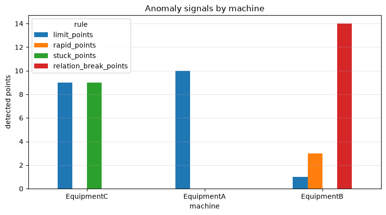
| EquipmentB | 1 | 3 | 0 | 14 | 19 | 67.40 | 4.22 |
/var/folders/3y/fmw40k0x78xblvb3gkcyvy1h0000gn/T/ipykernel_19414/1402267224.py:23: UserWarning: Glyph 35373 (\N{CJK UNIFIED IDEOGRAPH-8A2D}) missing from font(s) DejaVu Sans.
  plt.xticks(rotation=0); plt.tight_layout(); plt.show()
/var/folders/3y/fmw40k0x78xblvb3gkcyvy1h0000gn/T/ipykernel_19414/1402267224.py:23: UserWarning: Glyph 20633 (\N{CJK UNIFIED IDEOGRAPH-5099}) missing from font(s) DejaVu Sans.
  plt.xticks(rotation=0); plt.tight_layout(); plt.show()
/Users/hiroshi/private/kobo/notebook/.venv/lib/python3.13/site-packages/IPython/core/pylabtools.py:170: UserWarning: Glyph 35373 (\N{CJK UNIFIED IDEOGRAPH-8A2D}) missing from font(s) DejaVu Sans.
  fig.canvas.print_figure(bytes_io, **kw)
/Users/hiroshi/private/kobo/notebook/.venv/lib/python3.13/site-packages/IPython/core/pylabtools.py:170: UserWarning: Glyph 20633 (\N{CJK UNIFIED IDEOGRAPH-5099}) missing from font(s) DejaVu Sans.
  fig.canvas.print_figure(bytes_io, **kw)
Reading the results
Each piece of equipment has a different ‘type’ of abnormality. Equipment A focuses on sustained high temperatures, Equipment B focuses on sudden changes in vibration and relationship breakdown, and Equipment C focuses on pressure adhesion. In simple total rankings, long sticking tends to be overrated, so in practice, consecutive points are turned into events and prioritized by considering safety, quality, and downtime risks.
No.050: Interpreting Sensor Data Anomalies from the Field Perspective
Meaning in Practice
The analysis results do not end with “abnormal”; only when they translate who checks what, by when, and under what conditions driving continues or stops operation do they become valuable. Sensor and equipment abnormalities require different personnel and responses.
Approach to Analysis and Modeling
Assign causal hypotheses and recommended initial actions based on the rule combinations. This is not a confirmed fault diagnosis but triage. By adding equipment ledgers, maintenance history, operating status, and quality records, and recording the results after responses, rules and priorities are improved.
Check with Python
events = pd.DataFrame([
    ["EquipmentA", "Temperature exceeding the upper limit continues", "Insufficient cooling, overload, thermometer misalignment", "Check cooling flow rate and processing conditions. If the rise continues, decide to halt the plan.", "high"],
    ["EquipmentB", "Vibration spike/Relationship with electric current", "Impact, imbalance, tool wear, loose fixing", "Confirm the workpiece and tools, then re-measure with a portable vibration meter", "high"],
    ["EquipmentC", "Zero pressure sticking during operation", "Pressure sensor disconnection, communication disconnection, input card abnormality", "On-site instruments andPLCCompare values and inspect instrumentation systems.", "middle"],
], columns=["Equipment", "Summary of Detection", "Candidate cause", "Recommended initial move", "priority"])
display(events)

detected = df[["rapid_vibration", "pressure_zero_stuck", "any_limit_violation", "relation_break_flag"]].any(axis=1)
known = df.injected_event.ne("normal")
tp = int((detected & known).sum()); fp = int((detected & ~known).sum())
fn = int((~detected & known).sum())
print(f"Check point credits on the teaching materials: Detected abnormalities={tp}, Response to the Normal Point={fp}, Missed anomalies={fn}")| Equipment | Summary of Detection | Candidate cause | Recommended initial move | priority | |
|---|---|---|---|---|---|
| 0 | EquipmentA | Temperature exceeding the upper limit continues | Insufficient cooling, overload, thermometer misalignment | Check cooling flow rate and processing conditions. If the rise continues, decide to halt the plan. | high |
| 1 | EquipmentB | Vibration spike/Relationship with electric current | Impact, imbalance, tool wear, loose fixing | Confirm the workpiece and tools, then re-measure with a portable vibration meter | high |
| 2 | EquipmentC | Zero pressure sticking during operation | Pressure sensor disconnection, communication disconnection, input card abnormality | On-site instruments andPLCCompare values and inspect instrumentation systems. | middle |
Checking points in the textbook: Detected abnormal points = 33, Response to normal points = 2, Missed abnormalities = 1Reading the results
Equipment A covers process and cooling systems, Equipment B is mechanical, and Equipment C is instrumentation, resulting in different inspection routes. By converting responses from multiple rules into potential causes and initial responses, the distance from the monitoring screen to work instructions is shortened. Operational effectiveness is evaluated not only by point-level accuracy but also by whether failure events are captured in advance, whether average check times have shortened, or unnecessary stoppages have decreased.
Practical Implications Seen Through Target Exercise
- Distinguish data quality issues first: Inserting zero sticking or missing measurements into the equipment degradation model can lead to false learning.
- Combining physics and statistical rules: Safety limits serve immediacy, while relationship breakdowns serve early warning purposes.
- Manage by events, not points.: Summarizing consecutive anomalies by start, end, maximum, and duration is organized into cases on site.
- Standards for equipment and operating mode: Even for equipment of the same type, installation conditions and deterioration conditions differ, and uniform standards for all models increase false positives.
- Designing Cause Candidates and Recommended Initial Actions: Rather than the number of detections, KPIs include avoiding stoppages, reducing quality loss, and shortening inspection times.
What is necessary for practical implementation
- Data Contracts: Define tags, units, cycles, missing measurement codes, time synchronization, equipment/type, and operating status
- Approval of standards: Setting thresholds for alertness, abnormalities, and hazards based on manufacturer specifications, safety standards, process capabilities, and on-site knowledge
- Alert Operation: Define containment times, hysteresis, event integration, notification recipients, and escalation
- Verification Design: Evaluate not only past failures but also the man-hours required to confirm false positives and missed losses.
- Improvement Loop: Record the results of on-site inspections, causes, treatments, and replacement parts, and regularly review rules and models.
- System Integration: Connects with PLC/SCADA, Historian, MES, and CMMS to ensure permissions, audit logs, and availability.
If starting small, PoC is conducted based on 1 to 3 critical equipment units, one known failure mode, and rules that can be explained to the site, then the number of alerts and response flow are reviewed before expanding the scope.
Conclusion
From No.041 to No.050, we continuously checked everything from basic sensor data confirmation, sudden changes, zero adherence, upper and lower limits, correlations, relationship breakdowns, equipment comparisons, to on-site interpretation. The key is not to introduce advanced models first, but to Distinguishing between measurement anomalies and equipment anomalies, and connecting physically explainable detections to specific maintenance decisions..
Consultations for Corporations
At Mathematical Laboratory, we support everything from manufacturing data inventory, anomaly detection PoC, threshold and alert design, implementation into equipment maintenance systems, to on-site training, tailored to the challenges and data maturity. Even if you have data but don’t know which equipment or failure mode to start with, you can consult with us.
📩 Contact Us: surikobo.co.jp/contact
Please feel free to consult us first.