Don’t End Anomaly Detection with ‘Analysis’: 10 Practical Practices for Implementing and Operating Manufacturing Sites

This article covers the A seamless design method from model storage to on-site operation of abnormality detection in manufacturing equipment. Through No.091 to No.100, we verify reproducibility, batch processing, APIs, dashboards, on-site displays, model degradation, and the transition from PoC to production using fictional compressor equipment data.

[!NOTE] This material is a notebook previously used by Surikoubo (or personally by the representative, Kazuyama), and has been reconstructed, edited, and published with the company’s permission.
All data listed is fictional and has no relation whatsoever to real companies, factories, or figures.

Introduction: Practical Challenges in Manufacturing Covered in This Article

The value of anomaly detection does not come solely from creating highly accurate models. Only by applying the same preprocessing to new on-site data, reporting anomaly candidates to the responsible staff, recording response results, and monitoring performance changes can downtime losses and quality risks be reduced. This paper analyzes operational design that includes “who sees what, when, what they see, and how they make decisions.”

Common situations on site

• It works on the analyst’s PC but cannot be reproduced on the factory server.
• Column names, units, and missing items are handled differently for each CSV
• There are many alerts, but maintenance personnel cannot determine priorities.
• Failure to notice changes in equipment conditions after introduction leads to an increase in false positives.

Why is this issue so difficult to judge?

This is because model accuracy, downtime risk, response workload, system availability, and accountability all interact with each other. The abnormality score is not the failure probability itself; it also requires operational rules after exceeding the threshold. Therefore, technical KPIs and business KPIs are not separated, but managed within the same operational loop.

Overview of Exercise covered this time

No.	Theme	Operational deliverables
091–093	Save, Load, and New Inference	Reproducible models and inference results
094–095	Batch input/output	CSV processing and auditable results
096–097	API Dashboard	Points of contact with other systems and sites
098–099	On-site marking and deterioration monitoring	Prioritization and Relearning Decisions
100	From PoC to Production	Phased Implementation Roadmap

Preparing the Python environment

numpy, pandas, matplotlib, scikit-learn, and joblib are used. The API and screen examples also generate sources for FastAPI and Streamlit, but in this notebook, you don’t start the server and check syntax and deliverables. Random seed is fixed at 42.

from pathlib import Path
import json, sys
import joblib
import matplotlib
import matplotlib.pyplot as plt
import numpy as np
import pandas as pd
import sklearn
from sklearn.ensemble import IsolationForest
from sklearn.pipeline import Pipeline
from sklearn.preprocessing import StandardScaler

SEED = 42
rng = np.random.default_rng(SEED)
ARTIFACT_DIR = Path("artifacts_10")
ARTIFACT_DIR.mkdir(exist_ok=True)
pd.set_option("display.max_columns", 20)
plt.rcParams["figure.figsize"] = (10, 4)
print({"python": sys.version.split()[0], "pandas": pd.__version__,
       "scikit-learn": sklearn.__version__, "matplotlib": matplotlib.__version__})

{'python': '3.13.1', 'pandas': '3.0.3', 'scikit-learn': '1.9.0', 'matplotlib': '3.11.0'}

Creation of Fictional Data

Generates temperature, vibration, pressure, and load rate obtained every 10 minutes from three compressors. On the tail end, temperature and vibration drift and sudden abnormalities are mixed in, and the true_event is a fictitious label for explanation. For learning, only the first half, which is considered normal driving, is used.

n = 720
ts = pd.date_range("2026-04-01", periods=n, freq="10min")
equipment = np.resize(np.array(["CMP-01", "CMP-02", "CMP-03"]), n)
load = np.clip(rng.normal(72, 10, n), 35, 98)
temperature = 48 + 0.17 * load + rng.normal(0, 1.1, n)
vibration = 1.15 + 0.012 * load + rng.normal(0, 0.12, n)
pressure = 0.69 + 0.0018 * load + rng.normal(0, 0.012, n)
drift_idx = np.arange(n) >= 560
temperature[drift_idx] += np.linspace(0, 5.5, drift_idx.sum())
vibration[drift_idx] += np.linspace(0, 0.65, drift_idx.sum())
spikes = np.array([585, 632, 691, 708])
temperature[spikes] += [7, 9, 8, 10]
vibration[spikes] += [0.8, 1.0, 0.9, 1.2]
df = pd.DataFrame({"timestamp": ts, "equipment_id": equipment, "load_pct": load,
                   "temperature_c": temperature, "vibration_mm_s": vibration,
                   "pressure_mpa": pressure})
df["true_event"] = False
df.loc[spikes, "true_event"] = True
FEATURES = ["load_pct", "temperature_c", "vibration_mm_s", "pressure_mpa"]
display(df.head())
print("Number of lines:", len(df), "Number of explanatory events:", int(df.true_event.sum()))

	timestamp	equipment_id	load_pct	temperature_c	vibration_mm_s	pressure_mpa	true_event
0	2026-04-01 00:00:00	CMP-01	75.047171	60.652222	1.970811	0.818826	False
1	2026-04-01 00:10:00	CMP-02	61.600159	59.712848	1.932473	0.789553	False
2	2026-04-01 00:20:00	CMP-03	79.504512	59.006955	1.937172	0.848722	False
3	2026-04-01 00:30:00	CMP-01	81.405647	60.192657	2.299512	0.844131	False
4	2026-04-01 00:40:00	CMP-02	52.489648	55.908065	1.762592	0.791741	False

Number of lines: 720 Number of descriptive events: 4

No.091: Saving the Anomaly Detection Model

Meaning in Practice

Saving the model and preprocessing separately can cause mismatches in the order of transformation and parameters. Here, standardization and Isolation Forest are compiled into a Pipeline, and column names, thresholds, and library versions from training are also retained as metadata.

Approach to Analysis and Modeling

Inputs, models, thresholds, outputs, and monitoring indicators are treated as a single decision-making system. Not only accuracy but also reproducibility, processing time, explainability, man-hours addressed, and auditability are measured, and operational conditions are clearly defined.

Check with Python

train = df.iloc[:480].copy()
pipeline = Pipeline([("scaler", StandardScaler()),
                     ("model", IsolationForest(n_estimators=200, contamination=0.02,
                                               random_state=SEED, n_jobs=1))])
pipeline.fit(train[FEATURES])
train_scores = -pipeline.decision_function(train[FEATURES])
threshold = float(np.quantile(train_scores, 0.98))
model_path = ARTIFACT_DIR / "anomaly_pipeline.joblib"
meta_path = ARTIFACT_DIR / "model_metadata.json"
joblib.dump(pipeline, model_path)
meta = {"features": FEATURES, "threshold": threshold, "seed": SEED,
        "train_rows": len(train), "sklearn_version": sklearn.__version__}
meta_path.write_text(json.dumps(meta, ensure_ascii=False, indent=2), encoding="utf-8")
print(model_path, model_path.stat().st_size, "bytes")
print(meta)

artifacts_10/anomaly_pipeline.joblib 2412496 bytes
{'features': ['load_pct', 'temperature_c', 'vibration_mm_s', 'pressure_mpa'], 'threshold': 4.0766001685454967e-17, 'seed': 42, 'train_rows': 480, 'sklearn_version': '1.9.0'}

Reading the results

It is important not to limit the storage target to the “model itself” but to manage the input schema and judgment thresholds as the same version. This allows you to explain under what conditions alerts were issued during audits.

No.092: Loading the Saved Anomaly Detection Model

Meaning in Practice

The production process does not rerun the training code but loads approved deliverables. Performing feature matching and a simple smoke test immediately after loading allows for early detection of misplacement.

Approach to Analysis and Modeling

Inputs, models, thresholds, outputs, and monitoring indicators are treated as a single decision-making system. Not only accuracy but also reproducibility, processing time, explainability, man-hours addressed, and auditability are measured, and operational conditions are clearly defined.

Check with Python

loaded_pipeline = joblib.load(model_path)
loaded_meta = json.loads(meta_path.read_text(encoding="utf-8"))
assert loaded_meta["features"] == FEATURES
smoke_score = float(-loaded_pipeline.decision_function(df.loc[[0], FEATURES])[0])
print("Loading successful / Smoke Test Abnormal Score:", round(smoke_score, 4))

Loading success / Smoke test abnormality score: -0.2277

Reading the results

Loading success alone is not enough. By inspecting input columns, column order, units, missing tolerances, and model versions at deployment, data incidents before the model can be prevented.

No.093: Calculating Anomaly Scores for New Data

Meaning in Practice

Abnormal scores are stored as continuous values and separated from flags by thresholds. This is because the threshold can be revised later to match conservation capacity and missed loss costs.

Approach to Analysis and Modeling

Inputs, models, thresholds, outputs, and monitoring indicators are treated as a single decision-making system. Not only accuracy but also reproducibility, processing time, explainability, man-hours addressed, and auditability are measured, and operational conditions are clearly defined.

Check with Python

new_data = df.iloc[480:].copy()
new_data["anomaly_score"] = -loaded_pipeline.decision_function(new_data[FEATURES])
new_data["is_anomaly"] = new_data["anomaly_score"] >= loaded_meta["threshold"]
display(new_data.nlargest(8, "anomaly_score")[["timestamp", "equipment_id", "temperature_c",
        "vibration_mm_s", "anomaly_score", "is_anomaly", "true_event"]])
print("Number of Detected Cases:", int(new_data.is_anomaly.sum()))

	timestamp	equipment_id	temperature_c	vibration_mm_s	anomaly_score	is_anomaly	true_event
504	2026-04-04 12:00:00	CMP-01	54.209314	1.612695	0.099631	True	False
676	2026-04-05 16:40:00	CMP-02	68.965920	2.781650	0.094290	True	False
585	2026-04-05 01:30:00	CMP-01	68.771405	2.979259	0.081722	True	True
631	2026-04-05 09:10:00	CMP-02	67.648333	2.441341	0.078800	True	False
715	2026-04-05 23:10:00	CMP-02	63.442827	2.573856	0.067005	True	False
703	2026-04-05 21:10:00	CMP-02	66.631023	2.639065	0.060812	True	False
716	2026-04-05 23:20:00	CMP-03	62.494327	2.504022	0.051298	True	False
696	2026-04-05 20:00:00	CMP-01	63.451998	2.321404	0.048612	True	False

Number of detections: 38

Reading the results

Top candidates include artificially added spontaneous events. On the other hand, since gentle drifts are also detected, immediate stops and inspection reservations should not be treated the same way, but priority should be assigned to later stages.

No.094: Batch anomaly detection for CSV

Meaning in Practice

We assume operations where daily CSV deliveries from PLCs and data infrastructure. Processing functions check for required columns, types, and missing items, and in case of abnormalities, do not continue ambiguously and fail.

Approach to Analysis and Modeling

Inputs, models, thresholds, outputs, and monitoring indicators are treated as a single decision-making system. Not only accuracy but also reproducibility, processing time, explainability, man-hours addressed, and auditability are measured, and operational conditions are clearly defined.

Check with Python

input_csv = ARTIFACT_DIR / "incoming_sensor.csv"
new_data.drop(columns=["anomaly_score", "is_anomaly"]).to_csv(input_csv, index=False)

def score_csv(path, model, metadata):
    batch = pd.read_csv(path, parse_dates=["timestamp"])
    missing = sorted(set(metadata["features"]) - set(batch.columns))
    if missing:
        raise ValueError(f"No mandatory columns: {missing}")
    if batch[metadata["features"]].isna().any().any():
        raise ValueError("There are missing features")
    batch["anomaly_score"] = -model.decision_function(batch[metadata["features"]])
    batch["is_anomaly"] = batch["anomaly_score"] >= metadata["threshold"]
    return batch

batch_result = score_csv(input_csv, loaded_pipeline, loaded_meta)
print("Input:", input_csv, "Number of lines processed:", len(batch_result))

Input: artifacts_10/incoming_sensor.csv Number of lines processed: 240

Reading the results

The quality of batch processing depends not only on model accuracy but also on input inspection and failure notifications. In actual operation, file IDs, reception times, number of processing records, and error reasons are also recorded in the log.

No.095: Exporting Anomaly Detection Results to CSV

Meaning in Practice

The result files should be designed to be not only accessible by humans but also designed to be readable stably by subsequent processes. Adding model versions, check times, scores, and thresholds increases traceability.

Approach to Analysis and Modeling

Inputs, models, thresholds, outputs, and monitoring indicators are treated as a single decision-making system. Not only accuracy but also reproducibility, processing time, explainability, man-hours addressed, and auditability are measured, and operational conditions are clearly defined.

Check with Python

batch_result["model_version"] = "iforest-2026-04-v1"
batch_result["score_threshold"] = loaded_meta["threshold"]
batch_result["scored_at"] = pd.Timestamp("2026-04-06 00:00:00")
output_csv = ARTIFACT_DIR / "scored_sensor.csv"
batch_result.to_csv(output_csv, index=False, float_format="%.6f")
preview = pd.read_csv(output_csv, nrows=3)
display(preview)
print("exert effort:", output_csv, "Number of lines:", sum(1 for _ in output_csv.open()) - 1)

	timestamp	equipment_id	load_pct	temperature_c	vibration_mm_s	pressure_mpa	true_event	anomaly_score	is_anomaly	model_version	score_threshold	scored_at
0	2026-04-04 08:00:00	CMP-01	74.230797	59.164440	1.909521	0.830679	False	-0.190117	False	iforest-2026-04-v1	0.0	2026-04-06
1	2026-04-04 08:10:00	CMP-02	86.332145	62.141651	2.309214	0.844343	False	-0.134517	False	iforest-2026-04-v1	0.0	2026-04-06
2	2026-04-04 08:20:00	CMP-03	72.915202	60.857834	1.794402	0.809615	False	-0.172569	False	iforest-2026-04-v1	0.0	2026-04-06

Output: artifacts_10/scored_sensor.csv Lines: 240

Reading the results

To prevent duplicate handling even when reprocessing the same record, in practice, unique keys are created from the equipment ID and measurement time. CSV is convenient for handover, but if simultaneous updates or history management are needed, migrate to a database.

No.096: Creating an Anomaly Detection API with FastAPI

Meaning in Practice

With real-time integration, inference processing can be published as an HTTP API. It is important to include input validation, health checks, and model responses in the contract.

Approach to Analysis and Modeling

Inputs, models, thresholds, outputs, and monitoring indicators are treated as a single decision-making system. Not only accuracy but also reproducibility, processing time, explainability, man-hours addressed, and auditability are measured, and operational conditions are clearly defined.

Check with Python

api_source = """from fastapi import FastAPI
from pydantic import BaseModel, Field
import joblib, json, pandas as pd

app = FastAPI(title="Equipment Anomaly API", version="1.0.0")
model = joblib.load("artifacts_10/anomaly_pipeline.joblib")
meta = json.load(open("artifacts_10/model_metadata.json", encoding="utf-8"))

class SensorRecord(BaseModel):
    load_pct: float = Field(ge=0, le=100)
    temperature_c: float
    vibration_mm_s: float = Field(ge=0)
    pressure_mpa: float = Field(gt=0)

@app.get("/health")
def health(): return {"status": "ok", "model_version": "iforest-2026-04-v1"}

@app.post("/score")
def score(record: SensorRecord):
    x = pd.DataFrame([record.model_dump()])[meta["features"]]
    value = float(-model.decision_function(x)[0])
    return {"anomaly_score": value, "is_anomaly": value >= meta["threshold"]}
"""
api_path = ARTIFACT_DIR / "api_app.py"
api_path.write_text(api_source, encoding="utf-8")
compile(api_source, str(api_path), "exec")
print("FastAPIGenerated the source code and checked the syntax:", api_path)

Generated FastAPI source code and checked syntax: artifacts_10/api_app.py

Reading the results

API integration makes integration with MES and monitoring systems easier. However, timeouts, authentication, concurrency, input limits, log confidentiality, and model rolling updates must be designed separately.

No.097: Creating an Anomaly Detection Dashboard with Streamlit

Meaning in Practice

The dashboard is not a “place to view data,” but rather a business screen where the person in charge narrows down the inspection targets. Filter by equipment, duration, and priority, and simultaneously display the basis values and history.

Approach to Analysis and Modeling

Inputs, models, thresholds, outputs, and monitoring indicators are treated as a single decision-making system. Not only accuracy but also reproducibility, processing time, explainability, man-hours addressed, and auditability are measured, and operational conditions are clearly defined.

Check with Python

streamlit_source = """import streamlit as st
import pandas as pd

st.set_page_config(page_title="Equipment Abnormality Monitoring", layout="wide")
st.title("Equipment Abnormality Monitoring Dashboard")
df = pd.read_csv("artifacts_10/scored_sensor.csv", parse_dates=["timestamp"])
equipment = st.multiselect("Equipment", sorted(df.equipment_id.unique()), default=sorted(df.equipment_id.unique()))
view = df[df.equipment_id.isin(equipment)]
st.metric("abnormal candidate", int(view.is_anomaly.sum()))
st.line_chart(view.set_index("timestamp")[["anomaly_score", "score_threshold"]])
st.dataframe(view[view.is_anomaly].sort_values("anomaly_score", ascending=False))
"""
streamlit_path = ARTIFACT_DIR / "dashboard.py"
streamlit_path.write_text(streamlit_source, encoding="utf-8")
compile(streamlit_source, str(streamlit_path), "exec")
print("StreamlitGenerated the source code and checked the syntax:", streamlit_path)

Generated the Streamlit source and checked syntax: artifacts_10/dashboard.py

Reading the results

Count of cases KPIs alone does not lead to response decisions. It is important to be able to track equipment names, occurrence times, abnormality severity, related sensors, recommended actions, and corresponding status all in one screen.

No.098: Visualizing Anomaly Detection Results for the Field

Meaning in Practice

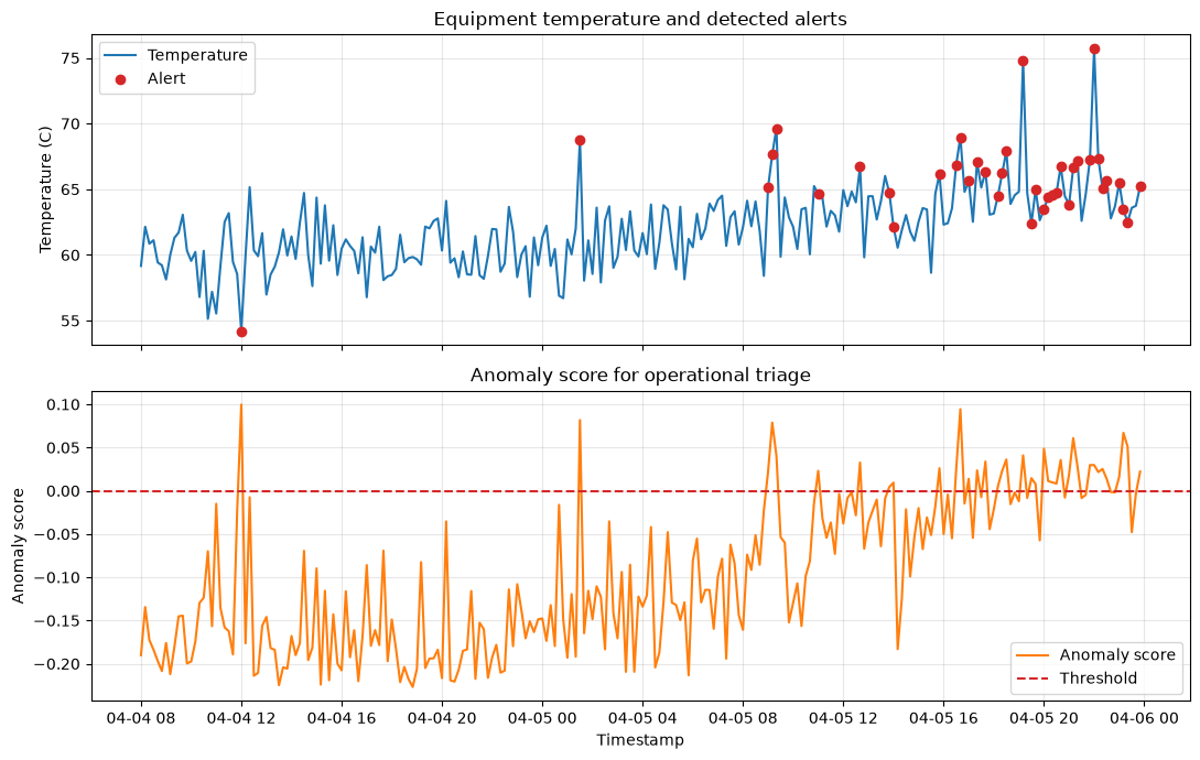
The on-site display shows not only abstract scores within the model but also which values of equipment deviate from the normal range. Here, we overlay time series, alert points, and thresholds.

Approach to Analysis and Modeling

Inputs, models, thresholds, outputs, and monitoring indicators are treated as a single decision-making system. Not only accuracy but also reproducibility, processing time, explainability, man-hours addressed, and auditability are measured, and operational conditions are clearly defined.

Check with Python

plot_df = batch_result.copy()
plot_df["priority"] = pd.cut(plot_df["anomaly_score"],
    bins=[-np.inf, loaded_meta["threshold"], loaded_meta["threshold"] + 0.04, np.inf],
    labels=["monitor", "inspect", "urgent"], right=False)
fig, axes = plt.subplots(2, 1, figsize=(11, 7), sharex=True)
axes[0].plot(plot_df.timestamp, plot_df.temperature_c, label="Temperature", color="#1f77b4")
alerts = plot_df[plot_df.is_anomaly]
axes[0].scatter(alerts.timestamp, alerts.temperature_c, color="#d62728", label="Alert", zorder=3)
axes[0].set(title="Equipment temperature and detected alerts", ylabel="Temperature (C)")
axes[0].grid(alpha=.3); axes[0].legend()
axes[1].plot(plot_df.timestamp, plot_df.anomaly_score, color="#ff7f0e", label="Anomaly score")
axes[1].axhline(loaded_meta["threshold"], color="#d62728", linestyle="--", label="Threshold")
axes[1].set(title="Anomaly score for operational triage", xlabel="Timestamp", ylabel="Anomaly score")
axes[1].grid(alpha=.3); axes[1].legend()
plt.tight_layout(); plt.show()
display(plot_df[plot_df.is_anomaly].groupby("priority", observed=True).size().rename("alerts").to_frame())

	alerts
priority
inspect	28
urgent	10

Reading the results

Because alerts are concentrated in the latter half, it is possible to suspect not only isolated failures but also changes in driving conditions or equipment condition. urgent is linked to immediate confirmation, inspect is for the next patrol, and monitor is for ongoing monitoring, all linked to response deadlines.

No.099: Considering Model Degradation and Retraining Timing

Meaning in Practice

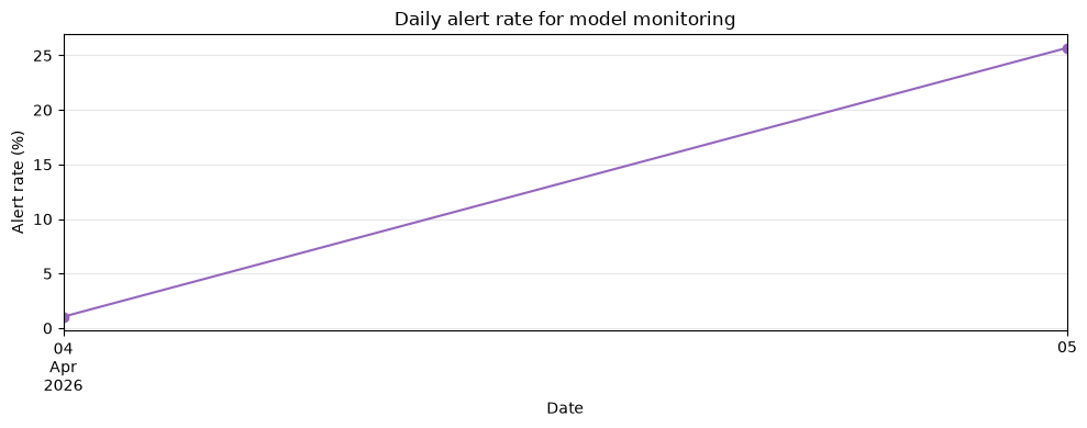
With unsupervised anomaly detection, the correct label does not align immediately. Therefore, changes in input distribution and alert rate are used as leading indicators, and after maintenance results are obtained, the accuracy rate and missed spots are checked. PSI measures the deviation between the ratio of bins during the reference period and the ratio during the monitoring period.

Approach to Analysis and Modeling

Inputs, models, thresholds, outputs, and monitoring indicators are treated as a single decision-making system. Not only accuracy but also reproducibility, processing time, explainability, man-hours addressed, and auditability are measured, and operational conditions are clearly defined.

Check with Python

def psi(reference, current, bins=10):
    edges = np.unique(np.quantile(reference, np.linspace(0, 1, bins + 1)))
    edges[0], edges[-1] = -np.inf, np.inf
    ref_p = pd.cut(reference, edges).value_counts(normalize=True, sort=False).clip(1e-6)
    cur_p = pd.cut(current, edges).value_counts(normalize=True, sort=False).clip(1e-6)
    return float(((cur_p - ref_p) * np.log(cur_p / ref_p)).sum())

monitor = df.iloc[480:].copy()
drift_report = pd.DataFrame({
    "feature": FEATURES,
    "psi": [psi(train[c], monitor[c]) for c in FEATURES]
})
drift_report["status"] = np.select([drift_report.psi >= .25, drift_report.psi >= .10],
                                   ["review", "watch"], default="stable")
display(drift_report.sort_values("psi", ascending=False))
weekly = batch_result.set_index("timestamp").resample("D")["is_anomaly"].mean().mul(100)
ax = weekly.plot(marker="o", color="#9467bd")
ax.set(title="Daily alert rate for model monitoring", xlabel="Date", ylabel="Alert rate (%)")
ax.grid(alpha=.3); plt.tight_layout(); plt.show()

	feature	psi	status
2	vibration_mm_s	0.970626	review
1	temperature_c	0.615939	review
3	pressure_mpa	0.080503	stable
0	load_pct	0.068061	stable

Reading the results

Increased temperature and vibration PSI and alert rates were the triggers for this review. However, if the change is legitimate due to seasonal or variety changes, stratification will be considered before relearning. Instead of “automatic relearning based on PSI exceedance,” it gates cause identification, data quality, label evaluation, and approval.

No.100: Organizing the Process from PoC to Production Implementation of the Anomaly Detection Project

Meaning in Practice

The purpose of a PoC is not to prove the highest accuracy, but to verify the operational value and feasibility of a production investment. Decide on end conditions, responsible persons, and operational KPIs for each stage.

Approach to Analysis and Modeling

Inputs, models, thresholds, outputs, and monitoring indicators are treated as a single decision-making system. Not only accuracy but also reproducibility, processing time, explainability, man-hours addressed, and auditability are measured, and operational conditions are clearly defined.

Check with Python

roadmap = pd.DataFrame([
 ["Issue Definition", "Agreed on Downtime Losses, Target Equipment, and Responders", "Business Manager", "delisted,80%explained with data"],
 ["Data Diagnosis", "Check quality, time synchronization, and history", "Data Officer", "missing mandatory items1%less than"],
 ["OfflinePoC", "Comparing Multiple Methods and Rules", "Analysis Specialist", "Once the situation is known,Recall 70%That's all."],
 ["Shadow Operations", "Scoring with actual data without notifying the site", "IT/preserve", "Processing success rate99%That's all."],
 ["Limited operation", "1Final decision on LINE", "Person responsible for preservation", "Effective Alert Rate50%That's all."],
 ["Production and Improvement", "Normalizing monitoring, auditing, and relearning", "Person in charge of operations", "Improved downtime and response times"],
], columns=["phase", "exit_criteria", "owner", "example_kpi"])
display(roadmap)
cost = pd.DataFrame({"scenario": ["Current Status", "Limited operation", "Production Operation"],
                     "annual_loss_million_yen": [24.0, 18.5, 13.0],
                     "annual_operating_cost_million_yen": [0.0, 2.5, 4.5]})
cost["total_million_yen"] = cost.annual_loss_million_yen + cost.annual_operating_cost_million_yen
display(cost)

	phase	exit_criteria	owner	example_kpi
0	Issue Definition	Agreed on Downtime Losses, Target Equipment, and Responders	Business Manager	delisted,80%explained with data
1	Data Diagnosis	Check quality, time synchronization, and history	Data Officer	missing mandatory items1%less than
2	OfflinePoC	Comparing Multiple Methods and Rules	Analysis Specialist	Once the situation is known,Recall 70%That's all.
3	Shadow Operations	Scoring with actual data without notifying the site	IT/preserve	Processing success rate99%That's all.
4	Limited operation	1Final decision on LINE	Person responsible for preservation	Effective Alert Rate50%That's all.
5	Production and Improvement	Normalizing monitoring, auditing, and relearning	Person in charge of operations	Improved downtime and response times

	scenario	annual_loss_million_yen	annual_operating_cost_million_yen	total_million_yen
0	Current Status	24.0	0.0	24.0
1	Limited operation	18.5	2.5	21.0
2	Production Operation	13.0	4.5	17.5

Reading the results

In this example, the total cost of production operations is lower than the current situation, but this is an estimate for assumption-based decision-making. In actual cases, we analyze sensitivity by setting avoidance stop time, false positive response time, implementation cost, and training cost in a range. Stage gates allow early stopping of investments whose value cannot be verified.

Practical Implications Seen Through Target Exercise

1. Models, preprocessing, feature schemas, thresholds, and edition information are managed in one unit.
2. Instead of turning abnormal scores into immediate stop orders, they convert into priority, response deadlines, and confirmation procedures.
3. Input/output inspection, logging, idempotence, and monitoring are set to the same quality requirements as model accuracy.
4. Changes in distribution are interpreted not as ‘evidence that the model is broken,’ but as signals to begin investigating the cause.
5. Production is not implemented all at once; instead, both technical and operational aspects are verified through shadow and limited operations.

What is necessary for practical implementation

• Business Design: Alert recipients, response deadlines, escalation, and record items
• Data Design: Equipment ID, time synchronization, unit, missing item, storage period, access rights
• System Design: Execution frequency, availability, authentication, logs, rollbacks, and failure notifications
• Evaluation Design: Missed and false positive costs, on-site inspection results, downtime losses, response time
• Governance: Model owner, change approval, version management, relearning conditions, audit trail

Conclusion

From No.091 to No.100, we confirmed the flow of saving anomaly detection models, applying them to new data, connecting them to operations via CSV, API, and dashboards, and gradually going live while monitoring degradation. The standard for success is not that the model is running, but that the site can make reasonable decisions with reasonable time and load, and continuously measure loss reduction.

Consultations for Corporations

At Suri Kobo, we support manufacturing companies tailored to their challenges and data maturity, covering everything from data diagnostics, anomaly detection PoC, evaluation design, to on-site operation and system implementation.

📩 Contact Us: surikobo.co.jp/contact
Please feel free to consult us first.