Advancing Quality Improvement with ‘Probability’: 10 Exercise-Keys to Bayesian Statistics for Manufacturing

In quality assurance, production technology, and equipment maintenance, even at stages with limited data, decisions must be made about “shipping,” “changing process conditions,” and “adding inspections.” In this article, we will examine the From the overall picture of Bayesian statistics to how to proceed with analysis projects in ten units numbered No.001 to No.010, using a fictional precision parts factory as the subject.

This “100 Exercises on Bayesian Statistics” series teaches you step by step, covering the basics of probability, Bayesian updates, Python calculations, estimation and forecasting, A/B testing, regression, hierarchical Bayes, business applications, and decision-making, all in line with manufacturing decision-making challenges. The goal is not to calculate the formula itself, but to Linking losses with actions while leaving uncertainty.

[!NOTE] This material is a notebook previously used by Surikoubo (or personally by the representative, Kazuyama), and has been reconstructed, edited, and published with the company’s permission.
All data listed is fictional and has no relation whatsoever to real companies, factories, or figures.

Introduction: Practical Challenges in Manufacturing Covered in This Article

In a hypothetical factory, the defect rate for precision parts after process changes is evaluated to ensure that the defect rate exceeds the management target 2%. Right after startup, the number of inspections is low, and even with zero defects, it cannot be definitively declared “safe.” On the other hand, postponing decisions increases losses due to full inspections, delivery delays, and stoppage losses.

The question in this article is not only the observed number of defects, but also how to communicate past insights with possible future outcomes to decision-makers.

Common situations on site

• Right after process changes or new equipment startup, with few specimens
• You have knowledge from past processes, but are unsure whether you can simply apply them to new processes.
• Only the average value or defect rate is reported, and the estimated range is not shared
• The cost and allowable risk of false positives differ among quality, production, and sales.

Why is this issue so difficult to judge?

The sample defect rate $x/n$ is a summary of observational results, not the true defect rate $p$ itself. Especially when the $n$ is small, random fluctuations are significant, and “zero defects” and “zero risk” do not coincide. Also, losses from misjudgments are asymmetric between shipment continuation and suspension. Therefore, it is necessary to address not only estimates but also $p$ uncertainties, the number of defective future lots, and judgment rules simultaneously.

Overview of Exercise covered this time

No.	Theme	Practical Questions
001	Overview of Bayesian Statistics	What to enter and what to judge
002	Differences from frequentism	How to explain the section
003	Treating uncertainty through probabilities	Several risks of exceeding targets
004	Pre-event, Likelihood, and Post-Event	How to integrate past insights with new data
005	Bayes Update	How to update test results each time
006	Data Growth and Belief	When data becomes dominant?
007	Point estimation and distribution estimation	What do you miss by just the average?
008	Forecast Values and Forecast Uncertainty	How many defective units will appear in the next lot
009	Points of Use	Which issues to introduce first
010	Analysis Project	Who decides what in the design

Preparing the Python environment

Only NumPy, pandas, SciPy, and matplotlib are used. The random number generator is fixed at seed=42 to allow the same results to be reproduced. SciPy’s beta is used to predict the pre- and post-defect rate distribution, while binom and betabinom are used to predict future defect numbers.

import platform
import numpy as np
import pandas as pd
import matplotlib
import matplotlib.pyplot as plt
import scipy
from scipy.stats import beta, binom, betabinom
from IPython.display import display

rng = np.random.default_rng(42)
plt.rcParams["figure.figsize"] = (8, 4.5)
plt.rcParams["axes.spines.top"] = False
plt.rcParams["axes.spines.right"] = False

print("Python     :", platform.python_version())
print("NumPy      :", np.__version__)
print("pandas     :", pd.__version__)
print("SciPy      :", scipy.__version__)
print("matplotlib :", matplotlib.__version__)

Python     : 3.13.1
NumPy      : 2.5.1
pandas     : 3.0.3
SciPy      : 1.18.0
matplotlib : 3.11.0

Creation of Fictional Data

The target is precision parts manufactured under new grinding conditions. Based on past similar processes, the preliminary distribution is set to $p\sim\mathrm{Beta}(2,98)$ (average 2%). In the new process, a total of 200 items were inspected over five days, generating hypothetical data showing that 4 defects were observed. Daily values are fixed for explanatory purposes and do not depend on external data.

daily = pd.DataFrame({
    "day": pd.date_range("2026-06-01", periods=5, freq="D"),
    "inspected": [40, 40, 40, 40, 40],
    "defects": [0, 1, 0, 2, 1],
})
daily["non_defects"] = daily["inspected"] - daily["defects"]
daily["observed_rate"] = daily["defects"] / daily["inspected"]

alpha0, beta0 = 2, 98
n = int(daily["inspected"].sum())
x = int(daily["defects"].sum())
alpha_post, beta_post = alpha0 + x, beta0 + n - x

display(daily.style.format({"observed_rate": "{:.1%}"}))
print(f"Total: {x} defects / {n} inspected = {x/n:.2%}")
print(f"Post-event distribution: Beta({alpha_post}, {beta_post})")

	day	inspected	defects	non_defects	observed_rate
0	2026-06-01 00:00:00	40	0	40	0.0%
1	2026-06-02 00:00:00	40	1	39	2.5%
2	2026-06-03 00:00:00	40	0	40	0.0%
3	2026-06-04 00:00:00	40	2	38	5.0%
4	2026-06-05 00:00:00	40	1	39	2.5%

Total: 4 defects / 200 inspected = 2.00%
Post-hoc distribution: Beta (6, 294)

No.001: Understanding What You Can Do with Bayesian Statistics

Meaning in Practice

Bayesian statistics connect past insights, new test results, and future forecasts through a single probabilistic model. The outputs include the “plausible range of the true defect rate,” the “probability of exceeding the target 2%,” and the “distribution of defect quantities in the next lot,” which directly serve as the basis for judgment in the quality meeting.

Approach to Analysis and Modeling

If the unknown defect rate is $p$, the number of observed defects is $x$, and the number of tests is $n$, then Bayesian inference

$p(p\mid x) \propto p(x\mid p)p(p)$

It can be expressed as such. The right side shows the likelihood of data occurrence, and the prior distribution, which represents the prior findings before observation. The posterior distribution on the left side is used for probability evaluation, prediction, and decision-making.

Check with Python

summary_001 = pd.DataFrame({
    "indicator": ["Observed rate", "Posterior mean", "P(rate > 2%)", "95% credible interval"],
    "value": [f"{x/n:.2%}", f"{alpha_post/(alpha_post+beta_post):.2%}",
              f"{1-beta.cdf(0.02, alpha_post, beta_post):.1%}",
              f"{beta.ppf(0.025, alpha_post, beta_post):.2%}–{beta.ppf(0.975, alpha_post, beta_post):.2%}"],
})
display(summary_001)

	indicator	value
0	Observed rate	2.00%
1	Posterior mean	2.00%
2	P(rate > 2%)	44.7%
3	95% credible interval	0.74%–3.86%

Reading the results

Even if the observation rate and the post-hoc average are close, looking at the probability of exceeding the target and the credit range can determine the accuracy of the judgment. By reporting not only the “estimated defect rate is about 2%” but also “how much possibility exceeds 2%,” it becomes possible to discuss additional inspections and provisional shipments.

No.002: Clarifying the Differences Between Frequency-Based Statistics and Bayesian Statistics

Meaning in Practice

The two are not superior; the questions they answer differ in their answers. The 95% confidence interval of frequentism is a procedural nature where, when the same procedure is repeated, 95% of the intervals cover the true value. The Bayesian 95% credit range can be interpreted as a 95% probability that $p$ is within the range under the model and data.

Approach to Analysis and Modeling

In frequentism, $p$ is treated as a fixed value, and data is treated as an amount that changes repeatedly. Bayesian statistics assign probability distributions to the $p$ after observation. Here, we compare the Wilson confidence interval with the Beta posterior credit interval. Due to the influence of prior distribution, Bayesian sections require the basis for pre-setting and sensitivity analysis.

Check with Python

z = 1.959963984540054
phat = x / n
center = (phat + z**2/(2*n)) / (1 + z**2/n)
half = z*np.sqrt(phat*(1-phat)/n + z**2/(4*n**2)) / (1 + z**2/n)
comparison = pd.DataFrame({
    "method": ["Frequentist: Wilson CI", "Bayesian: credible interval"],
    "lower": [center-half, beta.ppf(0.025, alpha_post, beta_post)],
    "upper": [center+half, beta.ppf(0.975, alpha_post, beta_post)],
    "interpretation": ["Coverage of repeated procedure", "Probability for parameter under model"],
})
display(comparison.style.format({"lower": "{:.2%}", "upper": "{:.2%}"}))

	method	lower	upper	interpretation
0	Frequentist: Wilson CI	0.78%	5.03%	Coverage of repeated procedure
1	Bayesian: credible interval	0.74%	3.86%	Probability for parameter under model

Reading the results

For minor defects, the lower and upper limits of the section vary depending on the method. In management reports, do not list only the numbers for the intervals; clearly state what is called probability. Designing a design that uses the estimation procedures for audit and standards compliance with the probability evaluation of operational decisions is also effective.

No.003: Understanding the Concept of Treating Uncertainty as Probability

Meaning in Practice

What the field often wants to know is not just “how many true values there are,” but “how likely they are to exceed the standard warning level.” The threshold exceedance probability can be used for rules for judging additional inspections or process stoppages.

Approach to Analysis and Modeling

By integrating $P(p>c\mid x)$ on the posterior distribution, we obtain the probability of exceeding any cautionary level $c$. However, statistics alone cannot determine what the probability of stopping is based on the probability. Decisions are made by combining outflow losses, downtime losses, safety, and customer requirements.

Check with Python

thresholds = np.array([0.01, 0.015, 0.02, 0.025, 0.03, 0.04])
exceedance = 1 - beta.cdf(thresholds, alpha_post, beta_post)

plt.plot(thresholds * 100, exceedance * 100, marker="o")
plt.title("Posterior exceedance probability")
plt.xlabel("Defect-rate threshold (%)")
plt.ylabel("P(rate exceeds threshold) (%)")
plt.grid(True, alpha=0.3)
plt.tight_layout()
plt.show()
display(pd.DataFrame({"threshold": thresholds, "exceedance_probability": exceedance})
        .style.format({"threshold": "{:.1%}", "exceedance_probability": "{:.1%}"}))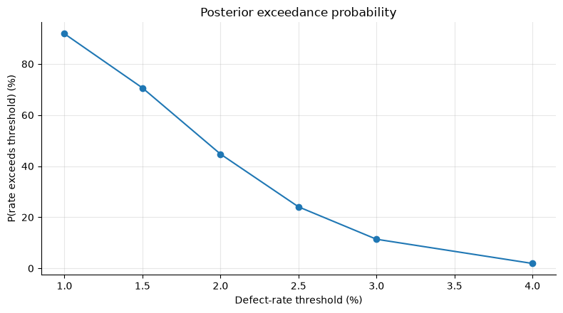

	threshold	exceedance_probability
0	1.0%	91.8%
1	1.5%	70.6%
2	2.0%	44.7%
3	2.5%	24.1%
4	3.0%	11.4%
5	4.0%	1.9%

Reading the results

The stricter the threshold, the higher the probability of exceeding it. In quality meetings, sharing this curve before it falls into a single “pass/fail” allows for visibility into which risks each department takes seriously.

No.004: Understanding the Relationship Between Prior Distribution, Likelihood, and Post-Distribution

Meaning in Practice

Ignoring past process performance makes estimation of small amounts of data unstable, and if you trust too much, you may miss anomalies after process changes. Prior distribution serves to turn ‘implicit rules of thumb’ into auditable values.

Approach to Analysis and Modeling

The binomial likelihood $x\sim\mathrm{Binomial}(n,p)$ and beta prior distribution $p\sim\mathrm{Beta}(\alpha_0,\beta_0)$ are conjugated,

$p\mid x\sim\mathrm{Beta}(\alpha_0+x,\beta_0+n-x)$

That’s how it works. $\alpha_0-1,\beta_0-1$ can intuitively be read as a pseudo-count of the past, but its precise interpretation depends on the method of presetting.

Check with Python

p_grid = np.linspace(0.0001, 0.08, 600)
prior_pdf = beta.pdf(p_grid, alpha0, beta0)
likelihood_scaled = binom.pmf(x, n, p_grid)
likelihood_scaled *= prior_pdf.max() / likelihood_scaled.max()
posterior_pdf = beta.pdf(p_grid, alpha_post, beta_post)

plt.plot(p_grid*100, prior_pdf, label="Prior: Beta(2, 98)")
plt.plot(p_grid*100, likelihood_scaled, "--", label="Likelihood (scaled)")
plt.plot(p_grid*100, posterior_pdf, label="Posterior: Beta(6, 294)")
plt.title("Prior, likelihood, and posterior")
plt.xlabel("Defect rate (%)")
plt.ylabel("Density / scaled likelihood")
plt.grid(True, alpha=0.3)
plt.legend()
plt.tight_layout()
plt.show()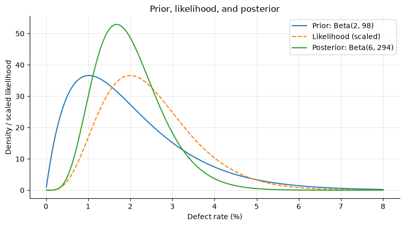

Reading the results

Post-posterior distributions are updated between past insights and current data. By using the pre-distribution, likelihood, and post-event distribution in the same diagram, the quality manager can check “how much experience was used.” The pre-distribution is not determined solely by the analyst; the definition of similar processes and the points for changes are agreed upon with the field team.

No.005: Understanding the Bayesian Renewal Concept

Meaning in Practice

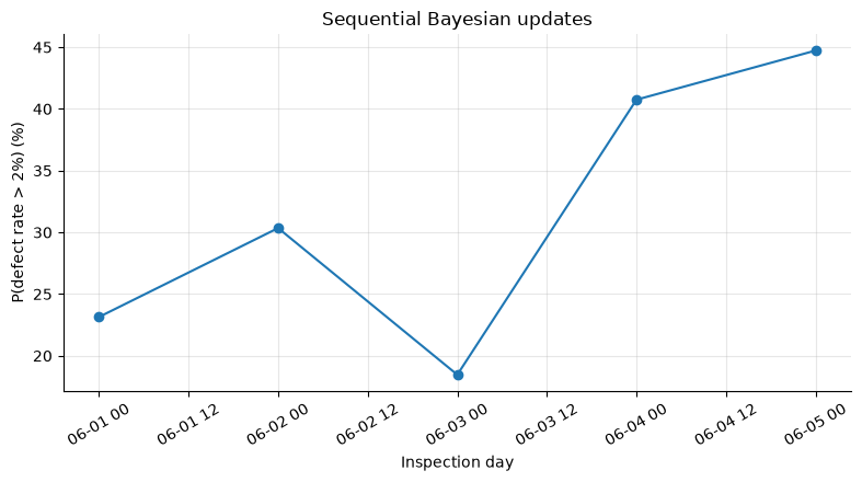
In sites where inspection data is delivered daily, updating the same rules sequentially under the same rules is more effective for early warning than to analyze everything at the end of the month. The post-distribution from the previous day can be reused as the pre-distribution for the next day.

Approach to Analysis and Modeling

The $t$ updates are $\alpha_t=\alpha_{t-1}+x_t$ and $\beta_t=\beta_{t-1}+n_t-x_t$. The results of a batch update and a sequential update match if the model is the same. In operations, data confirmation times, recalculations, and correction history are managed.

Check with Python

a, b = alpha0, beta0
rows = []
for row in daily.itertuples(index=False):
    a += int(row.defects)
    b += int(row.non_defects)
    rows.append({"day": row.day, "alpha": a, "beta": b,
                 "posterior_mean": a/(a+b), "p_over_2pct": 1-beta.cdf(0.02, a, b)})
updates = pd.DataFrame(rows)
display(updates.style.format({"posterior_mean": "{:.2%}", "p_over_2pct": "{:.1%}"}))

plt.plot(updates["day"], updates["p_over_2pct"]*100, marker="o")
plt.title("Sequential Bayesian updates")
plt.xlabel("Inspection day")
plt.ylabel("P(defect rate > 2%) (%)")
plt.grid(True, alpha=0.3)
plt.xticks(rotation=30)
plt.tight_layout()
plt.show()

	day	alpha	beta	posterior_mean	p_over_2pct
0	2026-06-01 00:00:00	2	138	1.43%	23.1%
1	2026-06-02 00:00:00	3	177	1.67%	30.3%
2	2026-06-03 00:00:00	3	217	1.36%	18.5%
3	2026-06-04 00:00:00	5	255	1.92%	40.7%
4	2026-06-05 00:00:00	6	294	2.00%	44.7%

Reading the results

On the day defects are observed, the probability of exceeding targets increases, and if good products continue, the rate decreases. It is important not to reflexively stop the game only with daily ups and downs; it is important to establish behavioral rules in advance, such as “the excess probability continuously exceeding the set value” or “expected loss exceeding the stop loss.”

No.006: Confirm the flow where beliefs are updated as data increases

Meaning in Practice

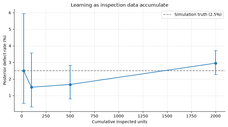
In the initial stages, past knowledge stabilizes the estimates, and as the number of inspections increases, the performance of new processes dominates the estimates. You can understand the value of additional testing and the process by which the impact of old findings fades.

Approach to Analysis and Modeling

Here, a reproducible fictitious series with a true defect rate of 2.5% is generated, and posterior distributions are compared by sample size. Post-variance shrinks as data increases, but if there is bias or dependence on data, information does not increase as much as simple sample size increases.

Check with Python

simulated = rng.binomial(1, 0.025, size=2000)
sample_sizes = [20, 100, 500, 2000]
learning = []
for size in sample_sizes:
    defects = int(simulated[:size].sum())
    a, b = alpha0 + defects, beta0 + size - defects
    learning.append({"n": size, "defects": defects, "mean": a/(a+b),
                     "lower": beta.ppf(.025, a, b), "upper": beta.ppf(.975, a, b)})
learning = pd.DataFrame(learning)
display(learning.style.format({"mean": "{:.2%}", "lower": "{:.2%}", "upper": "{:.2%}"}))

plt.errorbar(learning["n"], learning["mean"]*100,
             yerr=[(learning["mean"]-learning["lower"])*100,
                   (learning["upper"]-learning["mean"])*100], fmt="o-", capsize=4)
plt.axhline(2.5, color="gray", linestyle="--", label="Simulation truth (2.5%)")
plt.title("Learning as inspection data accumulate")
plt.xlabel("Cumulative inspected units")
plt.ylabel("Posterior defect rate (%)")
plt.grid(True, alpha=0.3)
plt.legend()
plt.tight_layout()
plt.show()

	n	defects	mean	lower	upper
0	20	1	2.50%	0.52%	5.94%
1	100	1	1.50%	0.31%	3.58%
2	500	8	1.67%	0.80%	2.83%
3	2000	60	2.95%	2.27%	3.72%

Reading the results

As the number of tests increases, the credit range narrows, reducing sensitivity to random fluctuations. However, 2,000 units with the same equipment and time slot may not represent the entire population. It is necessary to first organize stratification extraction and measurement system analysis.

No.007: Understanding the Difference Between Point Estimation and Distribution Estimation

Meaning in Practice

While point estimation is easy to include in KPI tables, it hides upside risk. Even with the same average of 2%, a wider distribution increases the risk of customer churn and the value of additional inspections.

Approach to Analysis and Modeling

Post-hoc means, medians, and MAP are representative values. When making decisions, both the credit band and the probability of exceeding the target are recorded. The MAP for the Beta$(a,b)$ is $(a-1)/(a+b-2)$ when it was $a,b>1$.

Check with Python

point_and_distribution = pd.DataFrame({
    "measure": ["Observed rate", "Posterior mean", "Posterior median", "MAP", "2.5% quantile", "97.5% quantile"],
    "estimate": [x/n, alpha_post/(alpha_post+beta_post), beta.median(alpha_post, beta_post),
                 (alpha_post-1)/(alpha_post+beta_post-2),
                 beta.ppf(.025, alpha_post, beta_post), beta.ppf(.975, alpha_post, beta_post)]
})
display(point_and_distribution.style.format({"estimate": "{:.2%}"}))

plt.fill_between(p_grid*100, posterior_pdf, alpha=0.25, label="Posterior uncertainty")
plt.plot(p_grid*100, posterior_pdf)
plt.axvline(alpha_post/(alpha_post+beta_post)*100, color="black", linestyle="--", label="Posterior mean")
plt.title("A point estimate inside a distribution")
plt.xlabel("Defect rate (%)")
plt.ylabel("Posterior density")
plt.grid(True, alpha=0.3)
plt.legend()
plt.tight_layout()
plt.show()

	measure	estimate
0	Observed rate	2.00%
1	Posterior mean	2.00%
2	Posterior median	1.89%
3	MAP	1.68%
4	2.5% quantile	0.74%
5	97.5% quantile	3.86%

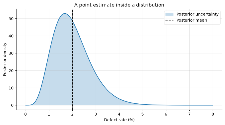
Reading the results

Even if representative values are close, the defect rate can be plausible. Including not only the posterior average but also the 95% credit range and excess probability on the dashboard makes it harder to overestimate the accuracy of the numbers.

No.008: Distinguishing Between Forecast Values and Forecast Uncertainty

Meaning in Practice

Estimating the defect rate parameter and predicting the actual number of defects in the next lot are two different things. The latter includes both parameter uncertainty and the chance of individual products defecting.

Approach to Analysis and Modeling

The next $m$ defective numbers $Y$ are binomial if $p$ are known, but integrating $p$ in posterior distribution yields a beta binomial distribution.

$P(Y=y\mid x)=\int P(Y=y\mid p)p(p\mid x)\,dp$

From this post-forecast distribution, we examine personnel, rework capacity, and delivery buffers.

Check with Python

future_n = 100
y = np.arange(0, 13)
predictive_pmf = betabinom.pmf(y, future_n, alpha_post, beta_post)
plugin_pmf = binom.pmf(y, future_n, alpha_post/(alpha_post+beta_post))
predictive_mean = future_n * alpha_post/(alpha_post+beta_post)
predictive_cdf = betabinom.cdf(np.arange(future_n+1), future_n, alpha_post, beta_post)
prediction_interval = (int(np.searchsorted(predictive_cdf, .025)), int(np.searchsorted(predictive_cdf, .975)))

plt.bar(y-0.18, predictive_pmf, width=0.36, label="Posterior predictive")
plt.bar(y+0.18, plugin_pmf, width=0.36, label="Plug-in binomial")
plt.title("Defects in the next 100-unit lot")
plt.xlabel("Number of defects")
plt.ylabel("Probability")
plt.grid(True, axis="y", alpha=0.3)
plt.legend()
plt.tight_layout()
plt.show()
print(f"Forecast Average: {predictive_mean:.2f}units")
print(f"95%Post-forecast Interval: {prediction_interval[0]}〜{prediction_interval[1]}units")
print(f"5Probability of more than one: {1-betabinom.cdf(4, future_n, alpha_post, beta_post):.1%}")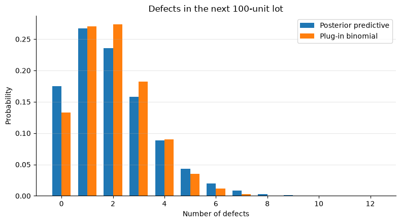

Forecast Average: 2.00
95% post-prediction intervals: 0 to 6 items
Probability of 5 or more: 7.6%

Reading the results

Even if the predicted average is about 2 lots, the actual next lot could be 0 or multiple lots. Compared to binomial distributions where parameters are fixed to the mean, the post-prediction distribution more broadly represents uncertainty. Instead of preparing an average of two rework personnel, you determine your remaining capacity based on the upper probability.

No.009: Organizing the Uses of Bayesian Statistics in Data Analysis

Meaning in Practice

Bayesian statistics are especially effective for tasks requiring small amounts of data, sequential judgment, information sharing between groups, and risk probability. On the other hand, models alone cannot solve the problem of broken data definitions.

Approach to Analysis and Modeling

Candidate projects are rated from 0 to 2 points on five perspectives: small data availability, continuous updates, past insights, loss asymmetry, and deployment value. This is not a statistical model, but a simple KPI that transparently prioritizes PoCs. Weights are agreed upon according to business policies.

Check with Python

candidates = pd.DataFrame({
    "use_case": ["New-process quality", "Predictive maintenance", "Demand planning", "Stable mass-production KPI"],
    "small_data": [2, 2, 1, 0], "sequential": [2, 2, 1, 1], "prior_knowledge": [2, 2, 1, 1],
    "asymmetric_loss": [2, 2, 2, 1], "scalability": [2, 1, 2, 1],
})
score_cols = ["small_data", "sequential", "prior_knowledge", "asymmetric_loss", "scalability"]
candidates["priority_score"] = candidates[score_cols].sum(axis=1)
candidates = candidates.sort_values("priority_score", ascending=False)
display(candidates)

plt.barh(candidates["use_case"], candidates["priority_score"])
plt.title("Bayesian PoC candidate score")
plt.xlabel("Priority score (0–10)")
plt.ylabel("Use case")
plt.grid(True, axis="x", alpha=0.3)
plt.gca().invert_yaxis()
plt.tight_layout()
plt.show()

	use_case	small_data	sequential	prior_knowledge	asymmetric_loss	scalability	priority_score
0	New-process quality	2	2	2	2	2	10
1	Predictive maintenance	2	2	2	2	1	9
2	Demand planning	1	1	1	2	2	7
3	Stable mass-production KPI	0	1	1	1	1	4

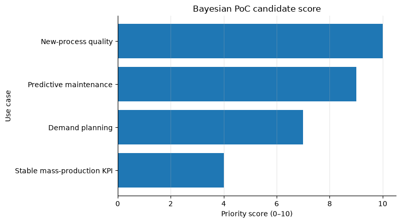
Reading the results

In this example, new process quality and predictive maintenance are the initial PoC candidates. However, a high score does not guarantee success. Add data acquisition costs, label quality, interventions that can be performed on site, and the presence or absence of responsible personnel as gate conditions.

No.010: Understanding the Process of Analysis Projects Using Bayesian Statistics

Meaning in Practice

The deliverable of analysis is not a “highly accurate model,” but a decision-making process that can be reproducible at the time of decision. We design objectives, data, models, validation, behavioral rules, and monitoring in sequence.

Approach to Analysis and Modeling

Projects are organized in the order of decision definition→ data audit→ pre-distribution agreement→ estimation and forecasting→ model checks→ decision rules including losses, → operational monitoring. At each stage, deliverables and approvers are assigned, and the conditions for re-approval when the model is changed are clearly defined.

Check with Python

project = pd.DataFrame({
    "step": [1, 2, 3, 4, 5, 6, 7],
    "phase": ["Decision", "Data audit", "Prior", "Inference", "Validation", "Decision rule", "Monitoring"],
    "deliverable": ["Action and loss table", "Data definition & MSA", "Prior rationale", "Posterior & prediction",
                    "Predictive checks", "Threshold & escalation", "Drift/review log"],
    "owner": ["Quality manager", "Data owner", "Domain + analyst", "Analyst", "Analyst + QA", "Plant manager", "Process owner"],
    "gate": ["Cost agreed", "Data accepted", "Sensitivity accepted", "Reproducible", "Fit for purpose", "Actionable", "Review cadence set"],
})
display(project.set_index("step"))

	phase	deliverable	owner	gate
step
1	Decision	Action and loss table	Quality manager	Cost agreed
2	Data audit	Data definition & MSA	Data owner	Data accepted
3	Prior	Prior rationale	Domain + analyst	Sensitivity accepted
4	Inference	Posterior & prediction	Analyst	Reproducible
5	Validation	Predictive checks	Analyst + QA	Fit for purpose
6	Decision rule	Threshold & escalation	Plant manager	Actionable
7	Monitoring	Drift/review log	Process owner	Review cadence set

Reading the results

Model building is part of seven stages. In particular, typical failures include moving forward with the measurement system unstable, deciding the prior distribution solely by the analyst, and not setting behavioral rules based on probability. Keeping approval records for each gate makes it easier to balance accountability and continuous improvement.

Practical Implications Seen Through Target Exercise

1. Report by distribution, not by a single point: Set the post-post average, 95% credit range, and the probability of exceeding the target.
2. Separate estimates from forecasts: Do not confuse the estimate of the true defect rate with the forecast of the number of defects in the next lot.
3. Controlling prior knowledge: Record the rationale, target period, similarity, and sensitivity analysis.
4. Translating Probability into Action: Define losses from stopping, additional inspections, and provisional shipments.
5. Don’t rely solely on data growth as a source of peace of mind: Monitor representativeness, measurement errors, and process changes.

What is necessary for practical implementation

• Inspection units, defect definitions, and traceability of lots, equipment, and materials
• Validation of measurement systems using Gage R&R and similar methods
• Evidence for prior distributions and sensitivity analysis using weak, standard, and strong prior distributions
• Post-forecast checks, outlier investigations, and model re-evaluation before and after process changes
• Judgment sheets including costs for misshipments, excessive stoppages, and additional inspections
• Operational design including update frequency, permissions, alerts, model versions, and approval history

Conclusion

From No.001 to No.010, Bayesian statistics were identified not only as a calculation method combining past insights with new data, but also as a framework for designing uncertain decisions in manufacturing sites. Rather than making definitive conclusions with a small amount of data, the key is to show the remaining risks in probabilities and turn them into actions through prediction and loss.

In the next phase, we will delve into the individual elements of the prior distribution, likelihood distribution, and post distribution, developing models that can handle differences among processes, equipment, and product groups.

Consultations for Corporations

At Mathematical Laboratory, we support issues from problem organization, data audits, PoC, decision-making rule design, to on-site training, covering areas such as quality improvement, equipment maintenance, and demand forecasting. You can consult with us from stages such as “too little data to analyze” or “unable to translate model results to on-site decisions.”

📩 Contact Us: surikobo.co.jp/contact
Please feel free to consult us first.