An introduction to factory simulation to avoid determining production capacity solely by “average”

The Overview and Purpose of 100 Exercises

“100 Exercises on Manufacturing Simulation” is a series that teaches you step by step, connecting probability distributions, queues, discrete events, continuous systems, stochastic processes, optimization, and digital twins to manufacturing decision-making. The goal is not to memorize techniques, but to acquire The ability to virtually compare measures such as capital investment, personnel allocation, inventory, and delivery dates before testing them on site.

This time, we will cover No.001 to No.010, “Introduction to Simulation.” Using a fictional assembly plant as a subject, we examine models, states, events, how time progresses, and the differences between probabilistic and deterministic models within the same operational context.

[!NOTE] This material is a notebook previously used by Surikoubo (or personally by the representative, Kazuyama), and has been reconstructed, edited, and published with the company’s permission.
All data listed is fictional and has no relation whatsoever to real companies, factories, or figures.

Introduction: Practical Challenges in Manufacturing Covered in This Article

At one assembly plant, a plan to increase orders is based on the average capacity of “100 units per day.” However, in reality, there are variations in processing times, sudden failures, scheduling, and fluctuations in demand. In this article, we consider whether delivery deadlines and work-in-progress (WIP) can be maintained even after increased production.

Common situations on site

• The average monthly production volume is within plan, but during busy days, the number of rigs surges
• Calculate capability based solely on average machining time, underestimating stoppages and variation.
• In Excel’s single scenario, the frequency of bad cases is unknown.
• The effects of equipment expansion, personnel support, and enhanced maintenance cannot be compared using the same KPI.

Why is this issue so difficult to judge?

Even if the average values are the same, differences in the order and variation of occurrence will affect the waiting time. Additionally, capital investment is expensive for testing actual machines, making it difficult to replicate conditions where congestion and breakdowns overlap. Simulation is an “experimental device for decision-making” that explicitly states assumptions and safely iterates multiple scenarios. However, a model is not the reality itself, but a simplified representation within the scope necessary for the purpose.

Overview of Exercise covered this time

No.	Theme	Questions in the Manufacturing Industry
001	What is Simulation?	Can measures be compared before introducing the actual equipment?
002	Why is it necessary?	What are the delivery risks that can’t be seen from the average?
003	System Modeling	What to leave behind and what to throw away from the factory
004	State variable	How to represent the current state of the factory?
005	Events	What events change the state?
006	Time Progression	How to choose between fixed cuts and event-driven
007	discrete time	How to track daily inventory and capacity
008	continuous time	How to track continuous volumes like tank water level
009	probability	How to measure risk, including variation,
010	determinism	How to check the reference case and sensitivity

Preparing the Python environment

No external data is used. numpy, pandas, and matplotlib generate and analyze fictional data. The random number generator fixes the seed so that rerunning it yields the same result.

import sys
import numpy as np
import pandas as pd
import matplotlib
import matplotlib.pyplot as plt
import japanize_matplotlib

SEED = 20260712
rng = np.random.default_rng(SEED)
pd.set_option("display.max_columns", 20)

print(f"Python     : {sys.version.split()[0]}")
print(f"numpy      : {np.__version__}")
print(f"pandas     : {pd.__version__}")
print(f"matplotlib : {matplotlib.__version__}")
print(f"random seed: {SEED}")

Python     : 3.13.1
numpy      : 2.5.1
pandas     : 3.0.3
matplotlib : 3.11.0
random seed: 20260712

Creation of Fictional Data

We assume an assembly line with 60 operating days. It generates demand, effective capacity, and downtime, and any insufficient inventory is carried over as a backlog to the next day. The figures here are for educational purposes and have no relation to actual factories.

n_days = 60
days = np.arange(1, n_days + 1)
demand = np.maximum(70, rng.normal(98, 13, n_days).round()).astype(int)
downtime = np.where(rng.random(n_days) < 0.18, rng.gamma(2.0, 1.1, n_days), 0.0)
capacity = np.maximum(65, (108 - 8.0 * downtime + rng.normal(0, 4, n_days)).round()).astype(int)

inventory, backlog = 120, 0
records = []
for day, dem, cap, stop in zip(days, demand, capacity, downtime):
    required = dem + backlog
    production = min(cap, required)
    available = inventory + production
    shipped = min(available, required)
    inventory = available - shipped
    backlog = required - shipped
    records.append((day, dem, cap, stop, production, shipped, inventory, backlog))

factory = pd.DataFrame(records, columns=[
    "day", "demand", "capacity", "downtime_h", "production", "shipped", "inventory", "backlog"
])
factory.head(10).round(2)

	day	demand	capacity	downtime_h	production	shipped	inventory	backlog
0	1	108	121	0.0	108	108	120	0
1	2	107	107	0.0	107	107	120	0
2	3	103	96	1.1	96	103	113	0
3	4	103	109	0.0	103	103	113	0
4	5	103	110	0.0	103	103	113	0
5	6	104	105	0.0	104	104	113	0
6	7	95	101	0.0	95	95	113	0
7	8	105	115	0.0	105	105	113	0
8	9	119	105	0.0	105	119	99	0
9	10	108	109	0.0	108	108	99	0

No.001: What is Simulation?

Meaning in Practice

Simulation is a method that reproduces the interactions of equipment, people, inventory, and orders on a computer and compares KPIs by measure. Rather than “guessing” the future with a single point, we examine what might happen when assumptions are set.

Approach to Analysis and Modeling

Here, we change capacity based on three options: current status, staff increase, and maintenance enhancement, and compare the maximum order backlog based on the difference between cumulative demand and cumulative production. The evaluation axis is not only average production volume but also the maximum order backlog, which directly affects service levels.

Check with Python

scenarios = {"Current Status": 0, "Increase in staff (+8platform/Day)": 8, "Enhanced security (halving stop)": None}
rows = []
for name, uplift in scenarios.items():
    cap = capacity + uplift if uplift is not None else np.maximum(65, (108 - 4.0 * downtime).round()).astype(int)
    daily_gap = demand - cap
    backlog_path = np.maximum.accumulate(np.r_[0, np.cumsum(daily_gap)])
    backlog_path = np.cumsum(daily_gap) - np.minimum.accumulate(np.r_[0, np.cumsum(daily_gap)])[:-1]
    rows.append([name, cap.mean(), max(0, backlog_path.max()), (cap >= demand).mean()])

scenario_result = pd.DataFrame(rows, columns=["policy", "average ability(platform/days)", "Maximum Order Backlog(platform)", "Daily Requirement Fulfillment Rate"])
scenario_result.round({"average ability(platform/days)": 1, "Daily Requirement Fulfillment Rate": 3})

	policy	average ability(platform/days)	Maximum Order Backlog(platform)	Daily Requirement Fulfillment Rate
0	Current Status	105.2	40	0.733
1	Increase in staff (+8platform/Day)	113.2	32	0.883
2	Enhanced security (halving stop)	106.6	28	0.817

Reading the results

The plan to uniformly increase capacity and reduce the impact of outages differs between the maximum backlog and daily demand fulfillment rate even if the average capacity is close. When making decisions, we check not only “how many vehicles have increased in average capacity,” but also whether delivery risk can be reduced within an acceptable range. By adding costs, you can then compare cost-effectiveness.

No.002: Why Simulation Is Necessary

Meaning in Practice

Even if average demand is below average capacity, if busy times and breakdowns overlap, backlogs will occur. Static ability tables cannot evaluate stagnation based on the order of occurrence.

Approach to Analysis and Modeling

Let the daily load rate be $\rho_t=D_t/C_t$. In addition to the average load rate, by looking at the upper quantile of the daily load rate and the time series of backorders, we evaluate by separating normal and harsh days.

Check with Python

factory["load_ratio"] = factory["demand"] / factory["capacity"]
summary_002 = factory[["demand", "capacity", "load_ratio", "backlog"]].agg(["mean", "max"])
display(summary_002.round(2))

fig, ax = plt.subplots(figsize=(9, 4))
ax.plot(factory["day"], factory["demand"], label="need", alpha=0.8)
ax.plot(factory["day"], factory["capacity"], label="effective capacity", alpha=0.8)
ax.fill_between(factory["day"], factory["capacity"], factory["demand"],
                where=factory["demand"] > factory["capacity"], color="tomato", alpha=0.25, label="insufficient ability")
ax.set_title("Daily demand and effective production capacity")
ax.set_xlabel("Operating Days")
ax.set_ylabel("platform/days")
ax.grid(True, alpha=0.3)
ax.legend()
fig.tight_layout()
plt.show()

	demand	capacity	load_ratio	backlog
mean	99.38	105.22	0.95	1.82
max	126.00	121.00	1.47	40.00

Reading the results

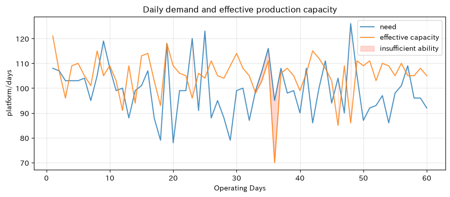
Even if the average for the entire period seems to have some capacity, in the red zone, the capacity on the day falls below demand. If such shortages continue, there will be backlog of orders until they can recover later. To determine delivery times, not only averages but also time series, maximum values, and upper quantiles are required.

No.003: What is System Modeling?

Meaning in Practice

System modeling is the process of defining scope, components, causality, and boundary conditions. When judging by increasing staff, the starting point is not to record all detailed human actions, but to preserve the relationships of capability, failure, demand, and inventory.

Approach to Analysis and Modeling

Assume the input is demand $D_t$ and capacity $C_t$, status is inventory $I_t$ and backorder $B_t$, and output is shipment $S_t$. Conceptually,

$I_{t+1}=\max(0, I_t+P_t-D_t-B_t), \qquad B_{t+1}=\max(0,D_t+B_t-I_t-P_t)$

That’s right. By removing unnecessary details from the objective, the model becomes explainable and easy to update.

Check with Python

model_register = pd.DataFrame({
    "Classification": ["Input", "Input", "Condition", "Condition", "Rules", "exert effortKPI"],
    "element": ["daily demand", "effective capacity", "Finished goods inventory", "unfinished order", "Inventory and Order Backlog Renewal Type", "Maximum Order Backlog"],
    "Unit": ["platform/days", "platform/days", "platform", "platform", "platform", "platform"],
    "Reason for keeping this time": ["Source of Load", "supply constraint", "He immediately contributed his remaining strength.", "Delivery risk", "Causality between elements", "Policy Comparison"]
})
model_register

	Classification	element	Unit	Reason for keeping this time
0	Input	daily demand	platform/days	Source of Load
1	Input	effective capacity	platform/days	supply constraint
2	Condition	Finished goods inventory	platform	He immediately contributed his remaining strength.
3	Condition	unfinished order	platform	Delivery risk
4	Rules	Inventory and Order Backlog Renewal Type	platform	Causality between elements
5	exert effortKPI	Maximum Order Backlog	platform	Policy Comparison

Reading the results

The model ledger clarifies “what to model and what hasn’t been added yet.” For example, since the product variety arrangement is not included, this model cannot be used as-is to make decisions where the variety composition strongly affects performance. Clearly stating the limits of the model is also part of quality.

No.004: What is a State Variable

Meaning in Practice

State variables are the information needed to resume future computations at a certain point in time. This includes inventory, order backlogs, equipment operating status, and work-in-progress.

Approach to Analysis and Modeling

By saving your condition daily, you can track the days when deterioration began and how long it took to recover. It is important not to confuse flow volume (demand and production) with stock volume (inventory and backlog of orders).

Check with Python

state_snapshot = factory.loc[factory["backlog"].idxmax(),
    ["day", "inventory", "backlog", "downtime_h", "capacity"]]
print("Status on the day the order backlog reached its maximum")
display(state_snapshot.to_frame("value").round(2))

fig, ax = plt.subplots(figsize=(9, 4))
ax.step(factory["day"], factory["inventory"], where="post", label="Finished goods inventory")
ax.step(factory["day"], factory["backlog"], where="post", label="unfinished order")
ax.set_title("Changes in factory state variables")
ax.set_xlabel("Operating Days")
ax.set_ylabel("platform")
ax.grid(True, alpha=0.3)
ax.legend()
fig.tight_layout()
plt.show()

Status on the day the order backlog reached its maximum

	value
day	48.00
inventory	0.00
backlog	40.00
downtime_h	2.47
capacity	86.00

Reading the results

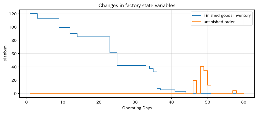
You can see the flow of backlog increasing after inventory decreases as buffer material. A snapshot of the maximum backlog dates serves as a starting point for analyzing causes not only by insufficient capacity but also by considering downtime and inventory levels up to the previous point.

No.005: What is an Event?

Meaning in Practice

Events are moments that instantly change the state, such as arrival, processing completion, breakdown, or recovery. Event history helps with accountability for stoppage losses and congestion.

Approach to Analysis and Modeling

Manage events using a table of “time, type, and state changes.” If there is a failure, the operating status is updated from 1 to 0; if recovered, it is updated from 0 to 1. Since the order affects the results, processing is done in chronological order.

Check with Python

events = pd.DataFrame([
    (0.0, "Start of business", 1, 0), (0.8, "Order Arrival", 0, 12), (1.6, "processing completed", 0, -1),
    (2.2, "equipment failure", -1, 0), (3.4, "Equipment restoration", 1, 0), (4.1, "processing completed", 0, -1),
    (5.0, "Order Arrival", 0, 8), (6.3, "processing completed", 0, -1),
], columns=["time(h)", "Events", "Changes in operating status", "Changes in waiting times"])
events["Operating status"] = events["Changes in operating status"].cumsum().clip(0, 1)
events["Waiting time"] = events["Changes in waiting times"].cumsum().clip(lower=0)
events

	time(h)	Events	Changes in operating status	Changes in waiting times	Operating status	Waiting time
0	0.0	Start of business	1	0	1	0
1	0.8	Order Arrival	0	12	1	12
2	1.6	processing completed	0	-1	1	11
3	2.2	equipment failure	-1	0	0	11
4	3.4	Equipment restoration	1	0	1	11
5	4.1	processing completed	0	-1	1	10
6	5.0	Order Arrival	0	8	1	18
7	6.3	processing completed	0	-1	1	17

Reading the results

The equipment condition is suspended from breakdown to recovery, but orders may arrive at different times. Although this example is simplified, in practice the rule is to reduce the waiting time after each processing completion and not trigger a completion event while the process is stopped. Event logs can explain in chronological order why the wait occurred.

No.006: Method of Time Progression

Meaning in Practice

How time is managed affects computational complexity and accuracy. Fixed time intervals are easy to understand as daily and minute-by-minute KPIs, while event-driven events are better suited for logistics and equipment behavior with irregular intervals.

Approach to Analysis and Modeling

The fixed increment method scans all time points. The event-driven system sends the clock forward to the next event time. The fewer events there are, the fewer times the latter process is processed.

Check with Python

horizon_min = 8 * 60
event_times = np.array([12, 48, 103, 177, 245, 332, 419, 475])
comparison = pd.DataFrame({
    "Method": ["Fixed Notch (1Minutes)", "Fixed Notch (10Minutes)", "Event-driven"],
    "clock update count": [horizon_min, horizon_min // 10, len(event_times)],
    "time expression": ["1by the minute", "10by the minute", "Keeping event times"],
    "Suitable Uses": ["Detailed continuous monitoring", "within the dayKPIEstimate", "Queues, malfunctions, and transport"]
})
comparison

	Method	clock update count	time expression	Suitable Uses
0	Fixed Notch (1Minutes)	480	1by the minute	Detailed continuous monitoring
1	Fixed Notch (10Minutes)	48	10by the minute	within the dayKPIEstimate
2	Event-driven	8	Keeping event times	Queues, malfunctions, and transport

Reading the results

Even with the same 8-hour cycle, the number of processing times can vary greatly. However, you shouldn’t choose based solely on the number of sessions. If you want to track continuous changes in temperature or liquid level, the validity of the notch width is important; if only processing completion or failure changes the state, event-driven action is natural.

No.007: Discrete-Time Simulation

Meaning in Practice

The discrete time model is well-suited for tasks that make decisions at regular intervals, such as daily inventory, weekly staff, and monthly supply and demand.

Approach to Analysis and Modeling

Update the day-end inventory to $I_{t+1}=\max(0,I_t+P_t-D_t)$ and count shortages as shortfalls. Since daytime variations shorter than the engraving width are not displayed, select the time granularity that fits your purpose.

Check with Python

weekly_demand = np.array([94, 106, 121, 88, 112, 97, 125, 101, 90, 116])
daily_capacity, stock = 105, 80
trajectory = []
for t, dem in enumerate(weekly_demand, 1):
    available = stock + daily_capacity
    shipped = min(available, dem)
    shortage = dem - shipped
    stock = available - shipped
    trajectory.append((t, dem, daily_capacity, shipped, stock, shortage))
discrete = pd.DataFrame(trajectory, columns=["days", "need", "Production", "Shipping", "day-end inventory", "missing item"])
discrete

	days	need	Production	Shipping	day-end inventory	missing item
0	1	94	105	94	91	0
1	2	106	105	106	90	0
2	3	121	105	121	74	0
3	4	88	105	88	91	0
4	5	112	105	112	84	0
5	6	97	105	97	92	0
6	7	125	105	125	72	0
7	8	101	105	101	76	0
8	9	90	105	90	91	0
9	10	116	105	116	80	0

Reading the results

Even with daily updates, you can see how inventory absorbs demand fluctuations. On the other hand, immediate delivery, where orders concentrate in the morning within the same day, cannot be evaluated. While it can be used for planning end-of-day inventory, evaluating wait times down to the minute requires a different granularity.

No.008: Continuous Time Simulation

Meaning in Practice

Quantities that continuously change over time, such as liquid level, temperature, pressure, and concentration, are represented by continuous-time models. It can be used for control settings and safety limit considerations.

Approach to Analysis and Modeling

The mixing tank water level $h(t)$ is set from the inflow $q_{in}$ and the outflow coefficient $k$

$\frac{dh}{dt}=q_{in}-kh$

Let’s say so. Here, we approximate using Euler’s $h_{t+\Delta t}=h_t+\Delta t(q_{in}-kh_t)$.

Check with Python

dt, end = 0.05, 12
t = np.arange(0, end + dt, dt)
h = np.zeros_like(t)
h[0] = 2.0
q_in, k = 0.8, 0.22
for i in range(len(t) - 1):
    h[i + 1] = h[i] + dt * (q_in - k * h[i])

fig, ax = plt.subplots(figsize=(8, 4))
ax.plot(t, h, label="Tank water level")
ax.axhline(q_in / k, color="tomato", linestyle="--", label="Theoretical equilibrium water level")
ax.set_title("Tank water level according to continuous time model")
ax.set_xlabel("hours (h)")
ax.set_ylabel("water level (m)")
ax.grid(True, alpha=0.3)
ax.legend()
fig.tight_layout()
plt.show()
print(f"12Water level after the time: {h[-1]:.2f} m / Equilibrium water level: {q_in/k:.2f} m")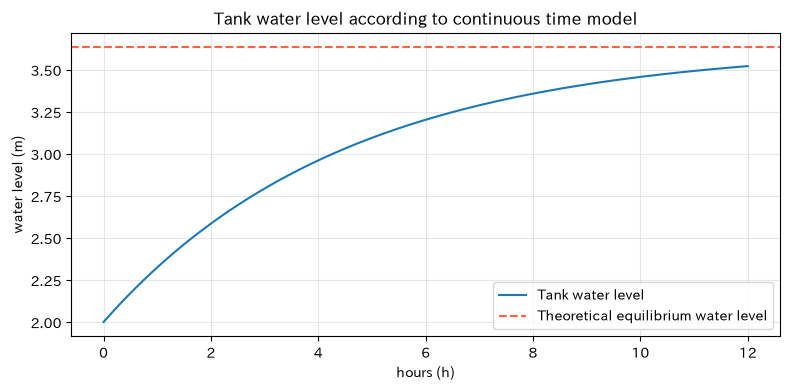

Water level after 12 hours: 3.52 m / Equilibrium level: 3.64 m

Reading the results

The water level does not immediately move to equilibrium but gradually approaches. If there is an upper water level, alarms and inflow control can be designed using the arrival time. In practical applications, coefficients are identified using measured values, and numerical errors are checked by varying the increment widths.

No.009: Probability Simulation

Meaning in Practice

Demand, breakdowns, and processing times can fluctuate by chance. Probabilistic simulation quantifies not only average results but also risks such as the probability of stockouts and lower percentiles of profits.

Approach to Analysis and Modeling

The Monte Carlo method is used, which involves repeating the same approach many times. Interests

$\text{interest}=1200\times\text{Shipment Volume}-400\times\text{Production Volume}-3000\times\text{Quantity of Units Out of Stock}$

Assume this and change the random number of demand and failure at each iteration. The amount is a relative comparative measure for teaching materials.

Check with Python

mc_rng = np.random.default_rng(SEED)
n_runs, horizon = 3000, 20
results = []
for run in range(n_runs):
    dem = np.maximum(0, mc_rng.normal(100, 14, horizon)).round()
    failures = mc_rng.binomial(1, 0.15, horizon)
    cap = 108 - failures * mc_rng.integers(20, 45, horizon)
    shortage = np.maximum(dem - cap, 0).sum()
    shipped = np.minimum(dem, cap).sum()
    profit = 1200 * shipped - 400 * cap.sum() - 3000 * shortage
    results.append((shortage, profit))
mc = pd.DataFrame(results, columns=["Total Shortage Units", "interest"])
metrics_009 = pd.Series({
    "Average out-of-stock quantity": mc["Total Shortage Units"].mean(),
    "Probability of out-of-stock occurrence": (mc["Total Shortage Units"] > 0).mean(),
    "interest5%point": mc["interest"].quantile(0.05),
    "average profit": mc["interest"].mean(),
})
display(metrics_009.to_frame("value").round(1))

fig, ax = plt.subplots(figsize=(8, 4))
ax.hist(mc["interest"] / 10000, bins=35, edgecolor="white")
ax.axvline(mc["interest"].quantile(0.05) / 10000, color="tomato", linestyle="--", label="interest5%point")
ax.set_title("20Simulated distribution of daily profits")
ax.set_xlabel("Profit (10,000 yen)")
ax.set_ylabel("Number of trials")
ax.grid(True, alpha=0.3)
ax.legend()
fig.tight_layout()
plt.show()

	value
Average out-of-stock quantity	115.1
Probability of out-of-stock occurrence	1.0
interest5%point	806540.0
average profit	1091632.2

Reading the results

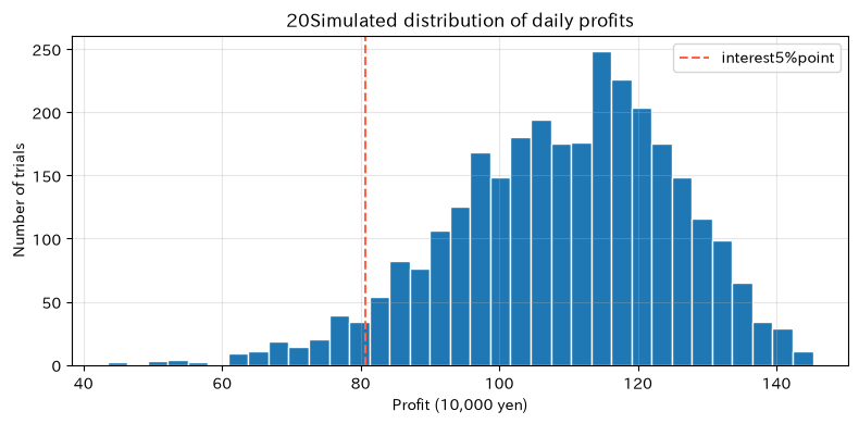
Average profits alone can miss out on losses in tough cases. The 5% profit point is a downside indicator, meaning “if the assumption is true, about 1 in 20 times it will be below this.” In management decisions, both expected values and risk tolerance are recorded, and distribution assumptions are verified using actual data.

No.010: Deterministic Simulation

Meaning in Practice

Deterministic models always return the same result for the same input. It is suitable for confirming alignment of baseline plans, explaining break-even points, and parameter sensitivity.

Approach to Analysis and Modeling

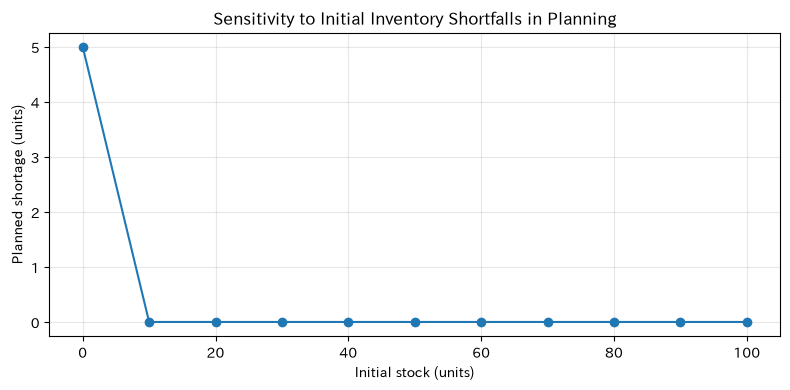
Fix demand and capacity, and only change safety stock levels. Instead of expressing uncertainty, the causality between input and result is clear. It is also effective as a comparison standard for probabilistic models.

Check with Python

demand_plan = np.array([95, 100, 110, 115, 105, 98, 120, 108, 102, 112])
capacity_plan = np.full_like(demand_plan, 106)
rows = []
for initial_stock in range(0, 101, 10):
    cumulative_net = initial_stock + np.cumsum(capacity_plan - demand_plan)
    min_stock = cumulative_net.min()
    shortage = max(0, -min_stock)
    ending_stock = cumulative_net[-1] + shortage
    rows.append((initial_stock, shortage, ending_stock))
deterministic = pd.DataFrame(rows, columns=["initial inventory", "Lack of planning", "End-of-period inventory after compensation"])
display(deterministic)

fig, ax = plt.subplots(figsize=(8, 4))
ax.plot(deterministic["initial inventory"], deterministic["Lack of planning"], marker="o")
ax.set_title("Sensitivity to Initial Inventory Shortfalls in Planning")
ax.set_xlabel("Initial stock (units)")
ax.set_ylabel("Planned shortage (units)")
ax.grid(True, alpha=0.3)
fig.tight_layout()
plt.show()

	initial inventory	Lack of planning	End-of-period inventory after compensation
0	0	5	0
1	10	0	5
2	20	0	15
3	30	0	25
4	40	0	35
5	50	0	45
6	60	0	55
7	70	0	65
8	80	0	75
9	90	0	85
10	100	0	95

Reading the results

You can explain the initial inventory threshold to eliminate shortages under a fixed plan. However, the probability of failures or demand fluctuations is unknown. First, a deterministic model is used to confirm the structure and reference values, and a step-by-step approach that probabilizes only important uncertainties is practical.

Practical Implications Seen Through Target Exercise

subject of judgment	Recommended expressions	Key KPIs	Points to Note
Monthly Supply and Inventory	Discrete Time and Determinism	Ending inventory and plan shortfall	You don’t see the crowds during the day.
Breakdown, transport, waiting	Event-driven and probabilistic	Wait times, WIP, and on-time delivery rates	Event rules need to be verified
Temperature, Liquid Level, and Pressure	continuous time	Time to reach the upper limit, stability value	Coefficient identification and indices check are necessary
capital investment	Multiple scenarios + probability	Expected profit, lower percentile, maximum order backlog	Include costs and constraints within the same boundary

The important thing is not to build advanced models from scratch. Decisions are made in advance, target KPIs, temporal granularity, and necessary states and events, then cultivated in a verifiable form from a simple deterministic model.

What is necessary for practical implementation

1. Defining decision-making: Clearly state options for comparison, such as equipment purchases, staffing support, and safety stock changes.
2. KPIand agree on acceptable values: Not only average, but also delivery on-time rates, maximum WIP, and 5% profit points, etc.
3. Check data quality: Define time, deceleration, stop reasons, and distinguish between planned and actual values.
4. Validate: Conduct on-site reviews, reproduce past periods, test extreme conditions, and conduct sensitivity analyses
5. Determine operational responsibilities: Updating assumptions, managing model versions, recalculating frequency, and determining approvers

Simulation results are not considered automatic decisions, but are presented to the decision-making meeting along with assumptions, scope of application, and uncertainty.

Conclusion

From No.001 to No.010, simulations were viewed as “experiments that express important real-world parts according to objectives and compare measures.” By distinguishing by status, event, and time progression method, you can choose models suitable for daily inventory, equipment failures, tank water levels, and more. Deterministic models indicate criteria and causality, while stochastic models indicate downside risk. In the next stage, we improve the model by cross-checking with actual results, connecting to decisions on investment, delivery times, and inventory.

Consultations for Corporations

At Suri Kobo, we support each stage of decision-making, from organizing data on the manufacturing site, designing simulations, comparing capital investment, personnel allocation, inventory measures, to in-house training. You can consult with us even at the stage of “first organizing the target process and KPIs.”

📩 Contact Us: surikobo.co.jp/contact
Please feel free to consult us first.